A new collection to be published by Scientific Reports on Ecological Networks has just been launched!
For this collection I will have the pleasure to be working with an excellent group of researchers and friends as a Guest Editor. The team includes Dr Isabel Donoso from the Basque Centre for Climate Change, Spain, Dr Sandra Hervías-Parejo and Dr Sérgio Timóteo from the University of Coimbra, Portugal, Dr Shai Pilosof, from Ben Gurion University of the Negev, Israel, Dr Irene Sagrera Mendoza, from the University of Sevilla, Spain, and myself.
It is very exciting to be part of this team as we hope to create a very nice collection of papers in one of our favourite research topics: Ecological Networks!
If you are working on something exciting right now, we are very much looking forward to your submission!
And please reach out if you have any questions.
Yesterday we had the pleasure to host Samraat, who visited us from Imperial College London to share his latest research on the coalescence of microbial communities with us at the Biomathematics Colloquium.
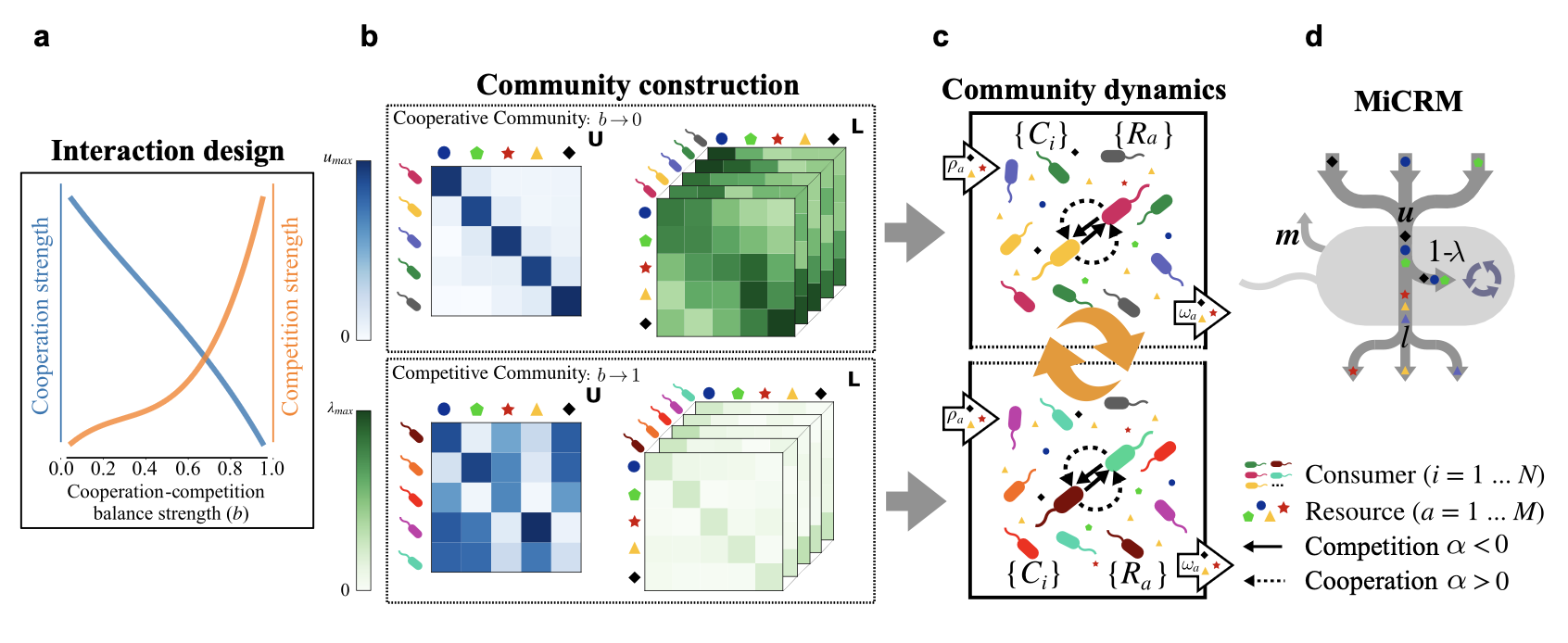
His talk, entitled Structural complementarity maximises feasibility and stability in microbial community coalescence summarised recent theoretical work using the Microbial Consumer-Resource Model MiCRM to investigate the possibility of predicting the composition and functionality of microbial communities that result from the coalescence of different assemblages. These assemblages may differ in the extent to which they harbour different interaction types from purely competitive to purely mutualistic communities. The composition of these interactions in parent communities then determines the outcome of the coalescence event and makes the final community predictable.
This theoretical work has many similarities with recent studies in our lab looking into the dynamics of microbial communities and has made us think about potential applications of our current work. These similarities and overlapping research interests yielded very interesting discussions afterwards that Samraat and I hope to keep alive by developing future joint collaborations and projects.
We also discussed potential new avenues with Jooyoung within the framework of her PhD project and how to potentially use a version of the MiCRM to increase the predictability of the role of microbial communities on the yield of red body in Nannochloropsis oceanica.
We ended the day at the pub for a pint and a nice meal! All in all a very interesting and productive visit. Thanks Samraat!
Picture credit: Zhu et al. (2026) bioRxiv
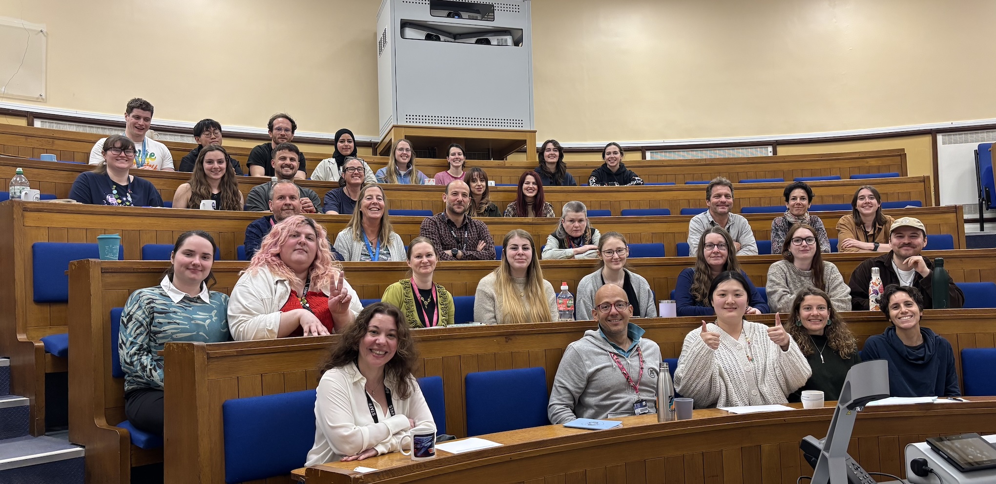
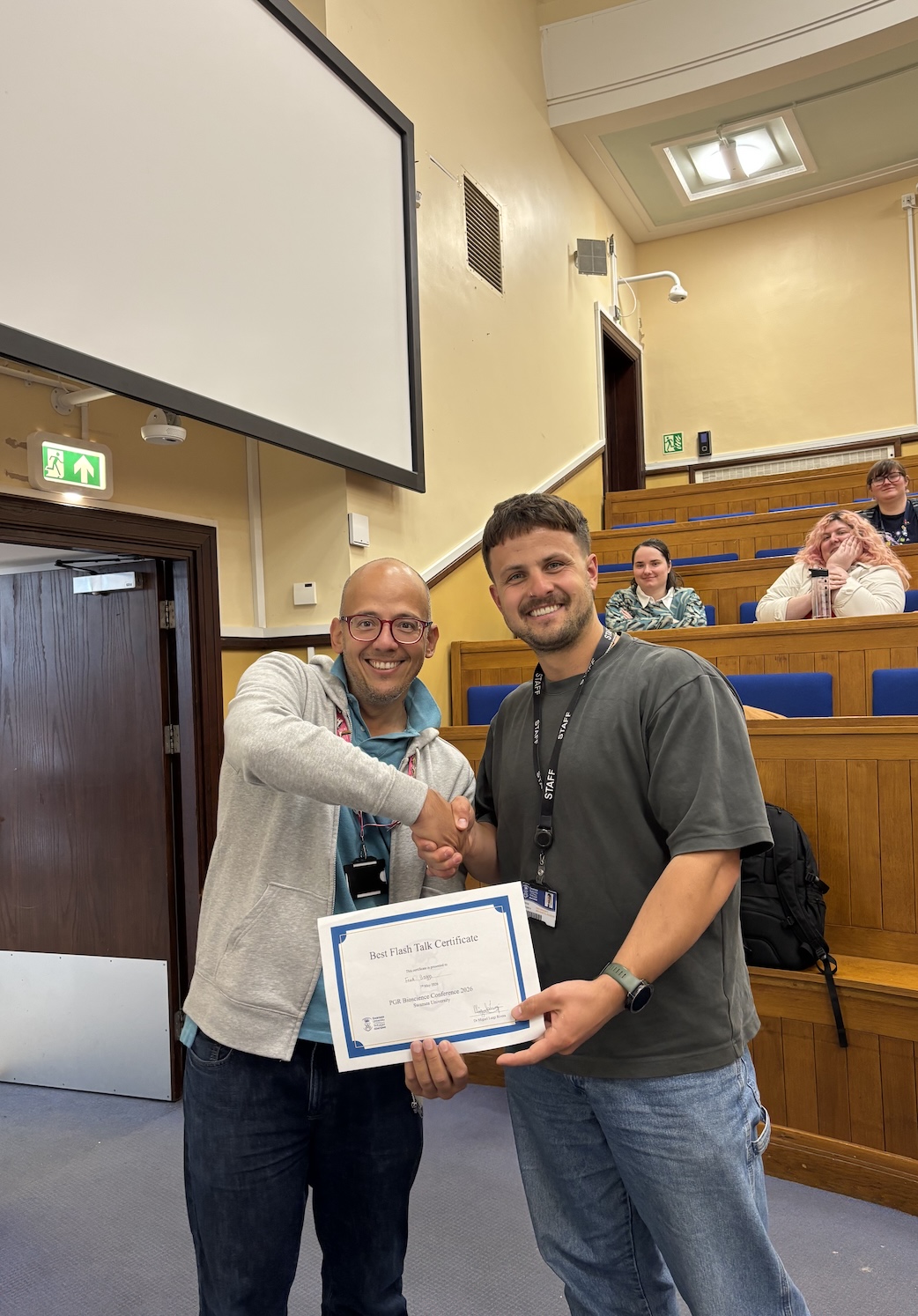
Last week we held the Annual Biosciences PGR conference, where postgraduate students at the Biosciences Department had the opportunity to present their latest research to an audience of fellow students and members of staff.
It was a great day packed with great presentations where we learnt about a diverse array of topics ranging from the harnessing of microbial communities to improve algal growth, to the understanding nutrient fluxes in marine forests, the effect of irrigation on sea turtle nest survival, and use of theoretical ecological models to improve restoration.
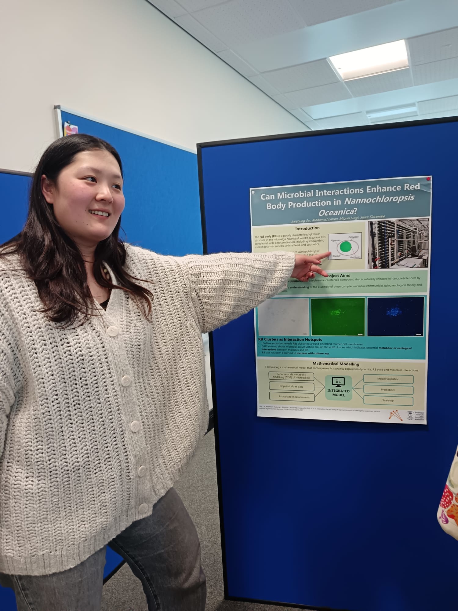
From the computational ecology lab, PhD students Jiacheng and Jooyoung presented their work on the modelling of restoration efforts in woodlands across Wales and the study of the role of microbial communities in the yield of red body production by Nannochloropsis oceanica algae.
Both students and members of staff in the audience posed great questions to the presenters which facilitated great discussions. These discussions were then taken to the poster session where we had the chance to learn more in detail about the work of some our MRes and PhD students on automated methods for detection of diseases in crabs to the use of engineered tiles to improve grazing by limpets of macroalgae as a biological solution to biofouling.
At the end of the day all conference attendees voted for their favourite talks and posters and the winning students received some amazing prizes arranged by the organisers.
Special thanks go to Jooyoung and Lucia who organised the entire conference, from putting together the programme, to coordinating prizes and coffee breaks, make the whole event possible.
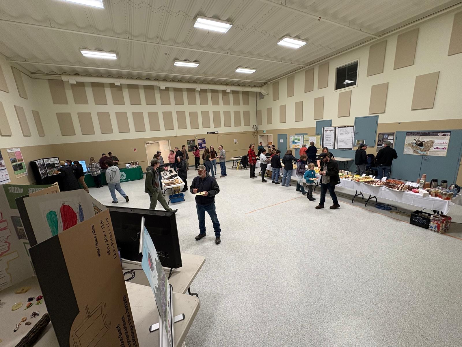
Last week I had the pleasure to contribute to The John Prince Research Forest’s community Open House event at Fort St. James, Canada.
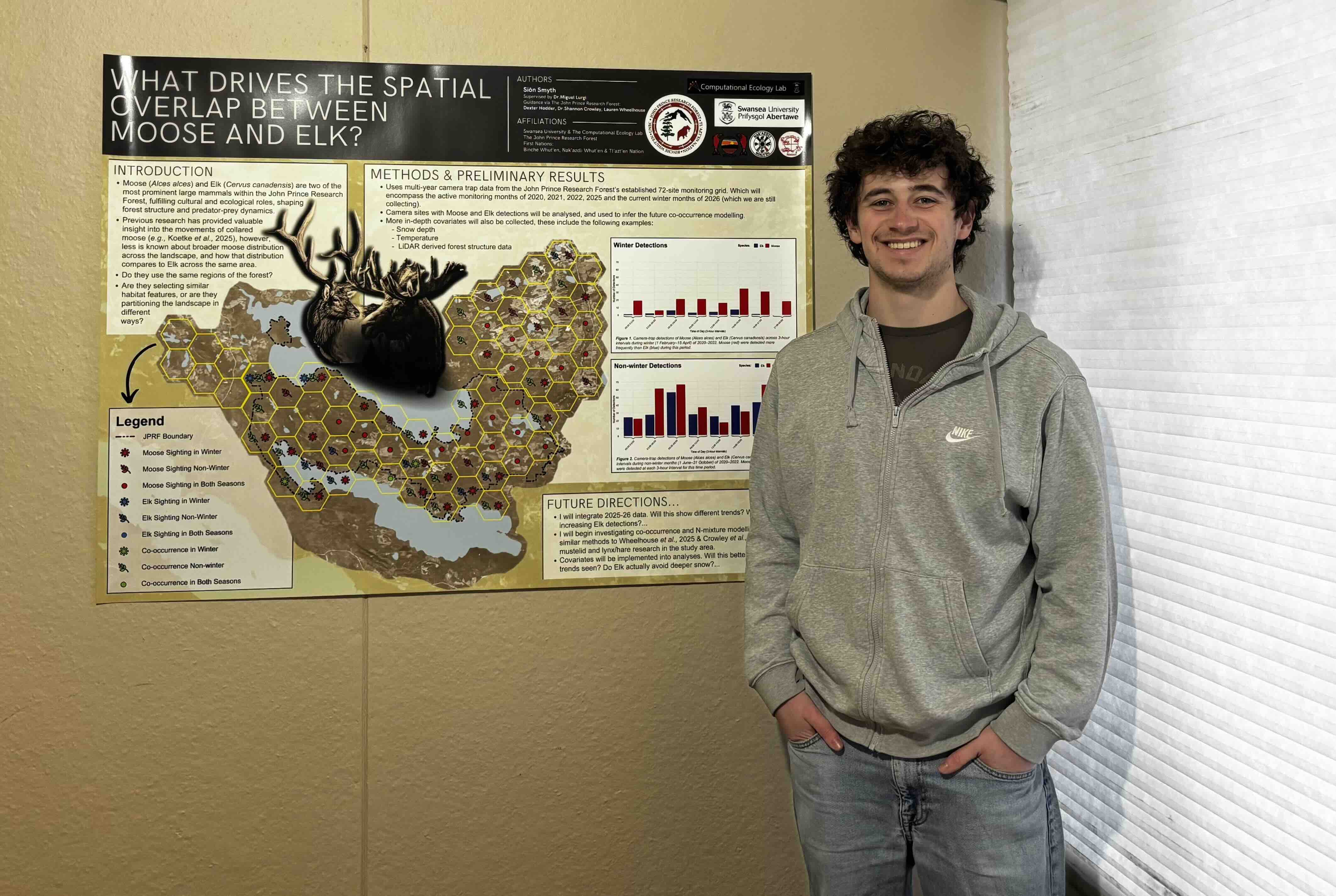
The event welcomed everyone from the surrounding communities and a-far to learn more about the ongoing and past research done at the organisation. This included countless research projects taken on by students, including my own; What drives the spatial overlap between moose and elk?
It was great to be able to discuss my project with the local community, and to learn more from them about the surrounding area. With affiliated researchers and students to the John Prince Research Forest in attendance, discussions about the huge diversity of projects being conducted at the study area was far from scarce.
Overall a fantastic evening!

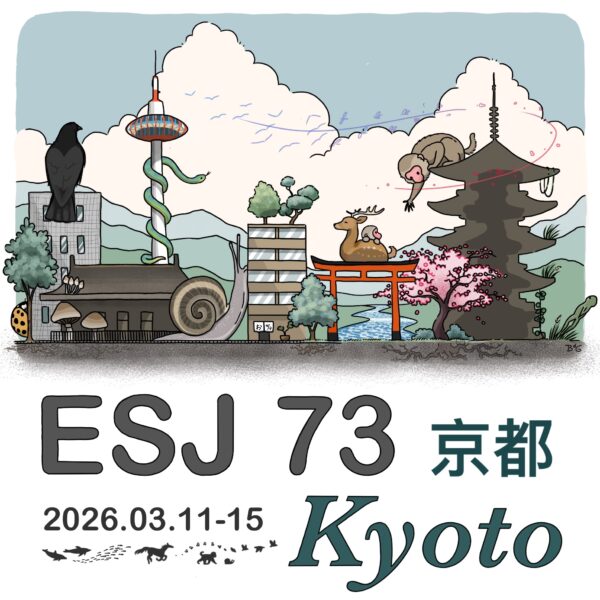
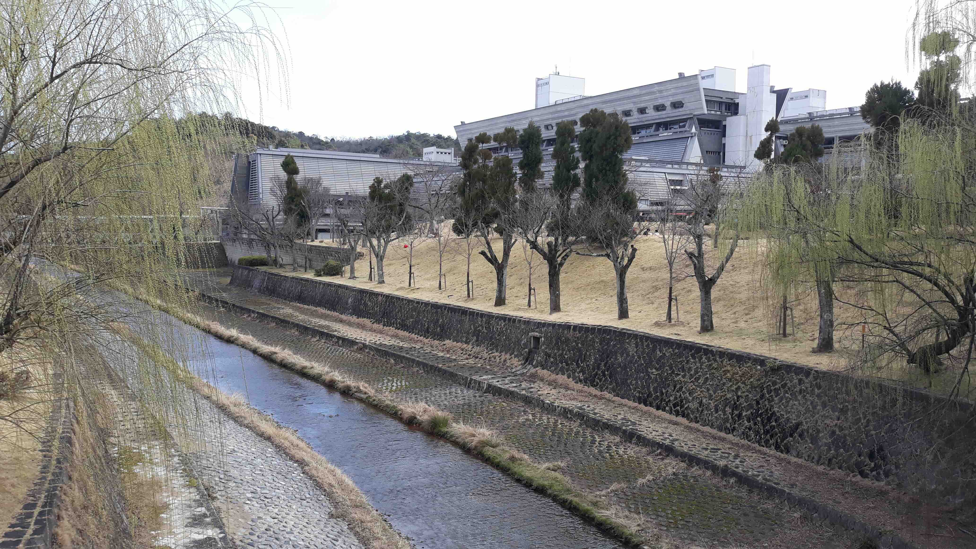
Last week I attended for the first time the Annual Meeting of the Ecological Society of Japan in Kyoto. It was a very interesting conference with many presentations ranging from theoretical ecology to biodiversity and conservation, and the latest findings on biodiversity-stability relationships.
The conference was held in 2 different venues, which was great to explore different parts of the city of Kyoto. The first part of the conference was held in the Yoshida-South Campus of the University of Kyoto. A very nice student-vibe atmosphere with lots going on in the surroundings and close to the Kyoto river.
Towards the end we moved to the Kyoto International Conference Centre, where the poster session took place and provided a great opportunity to chat to different students about their current projects and browse around many interesting projects going on across Japan.