Two new exciting opportunities for PhD scholarships just went live today on projects related to restoration ecology using quantitative mechanistic models of species distributions and interaction networks. Closing date the 30th of June. So hurry up! Check out our join page for full details!
News from the Computational Ecology Lab
New PhD positions advertised!
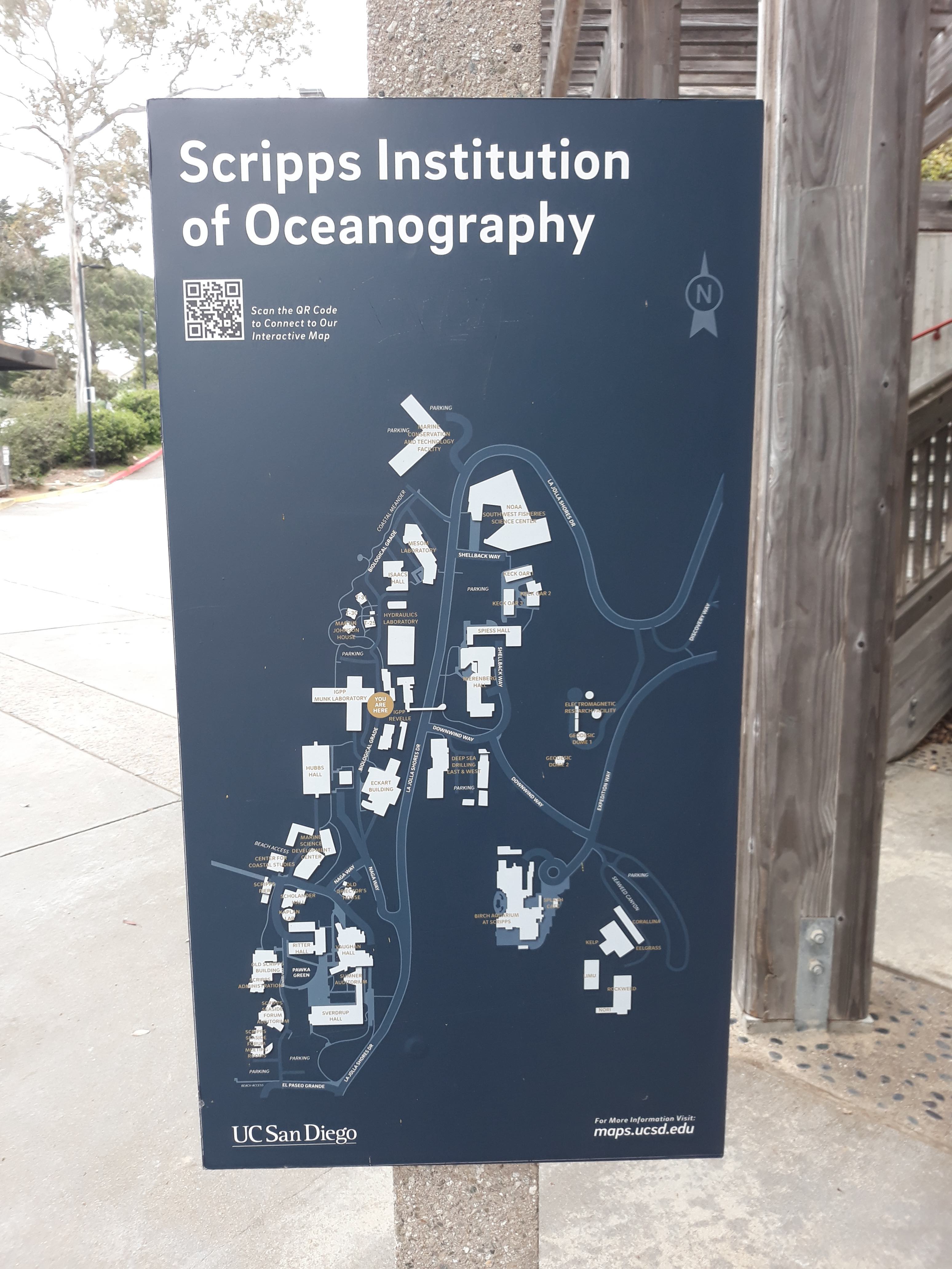
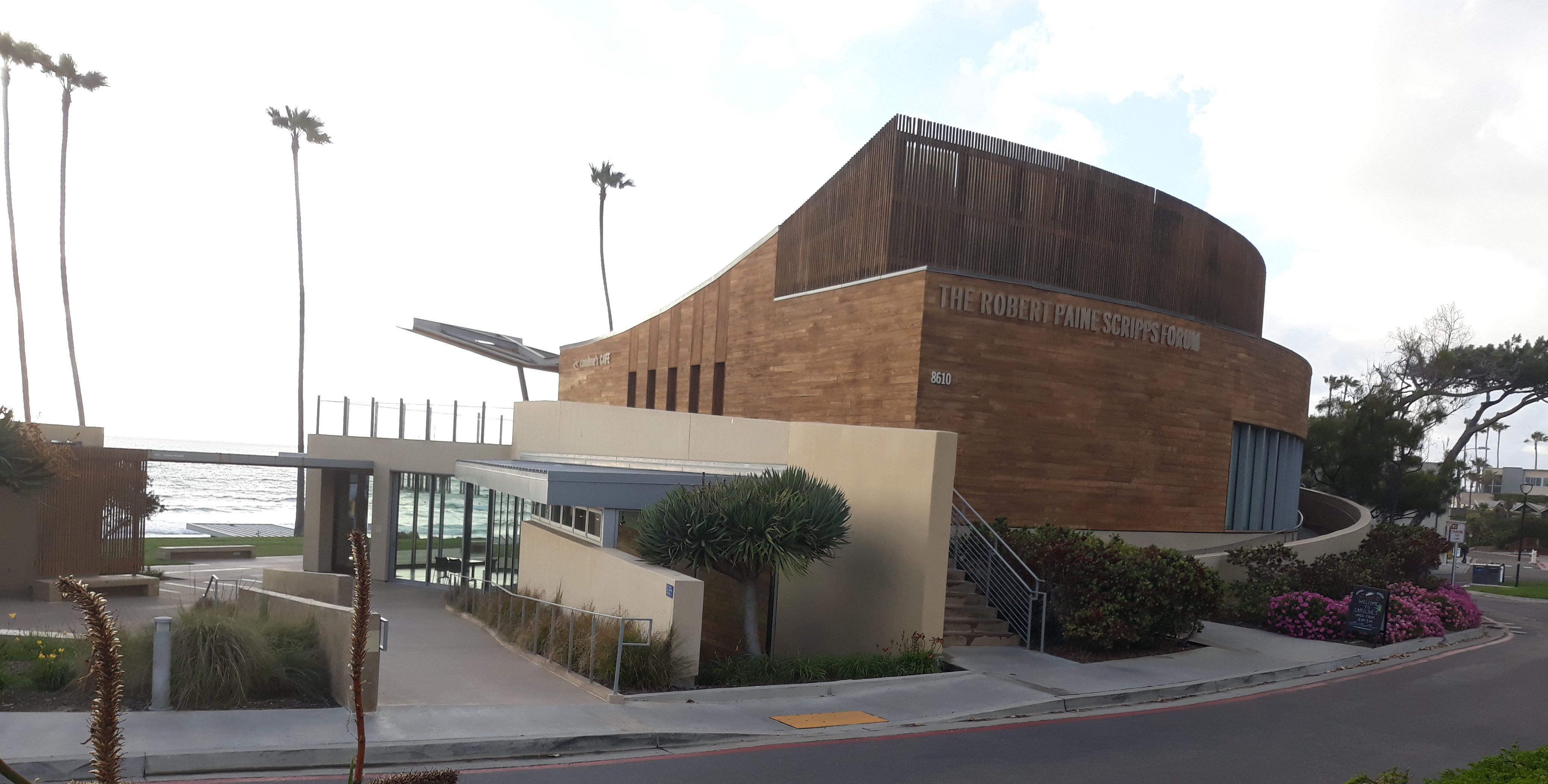
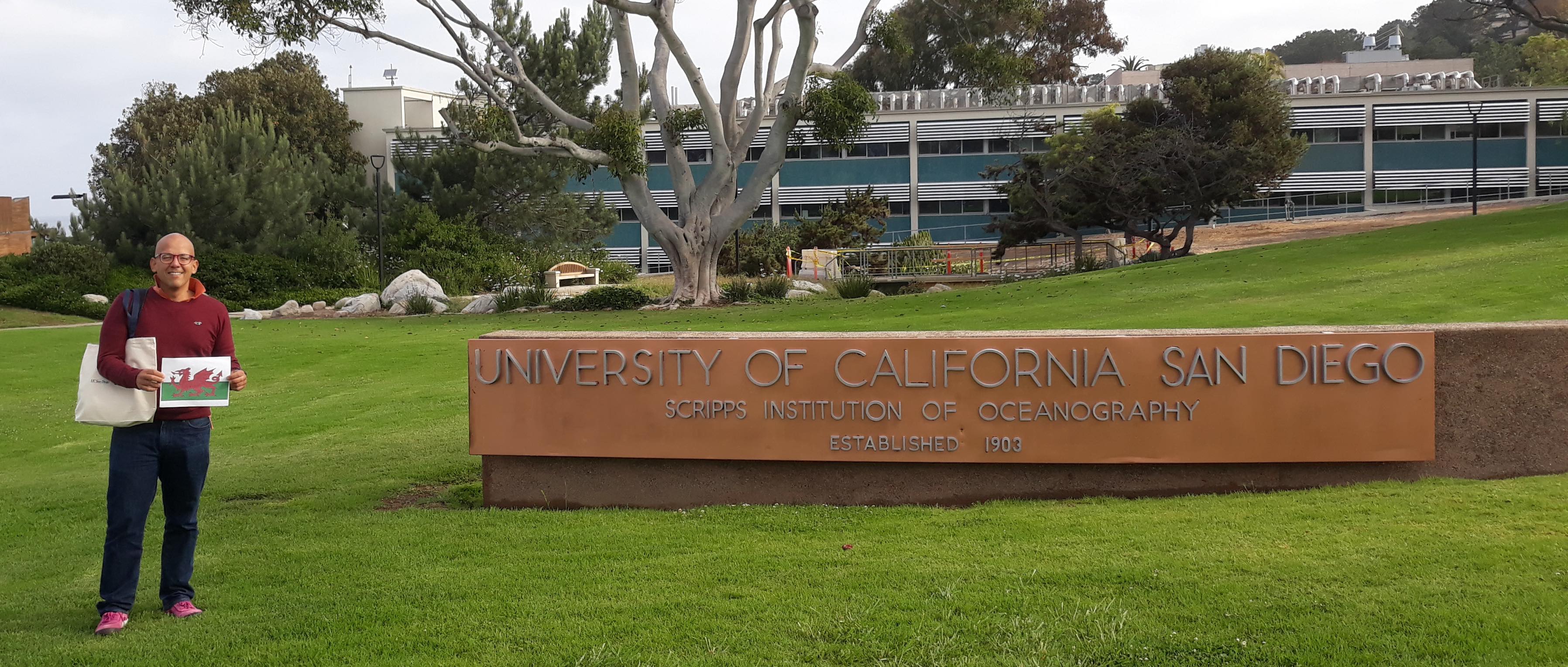
Research visit to the Scripps Institution of Oceanography
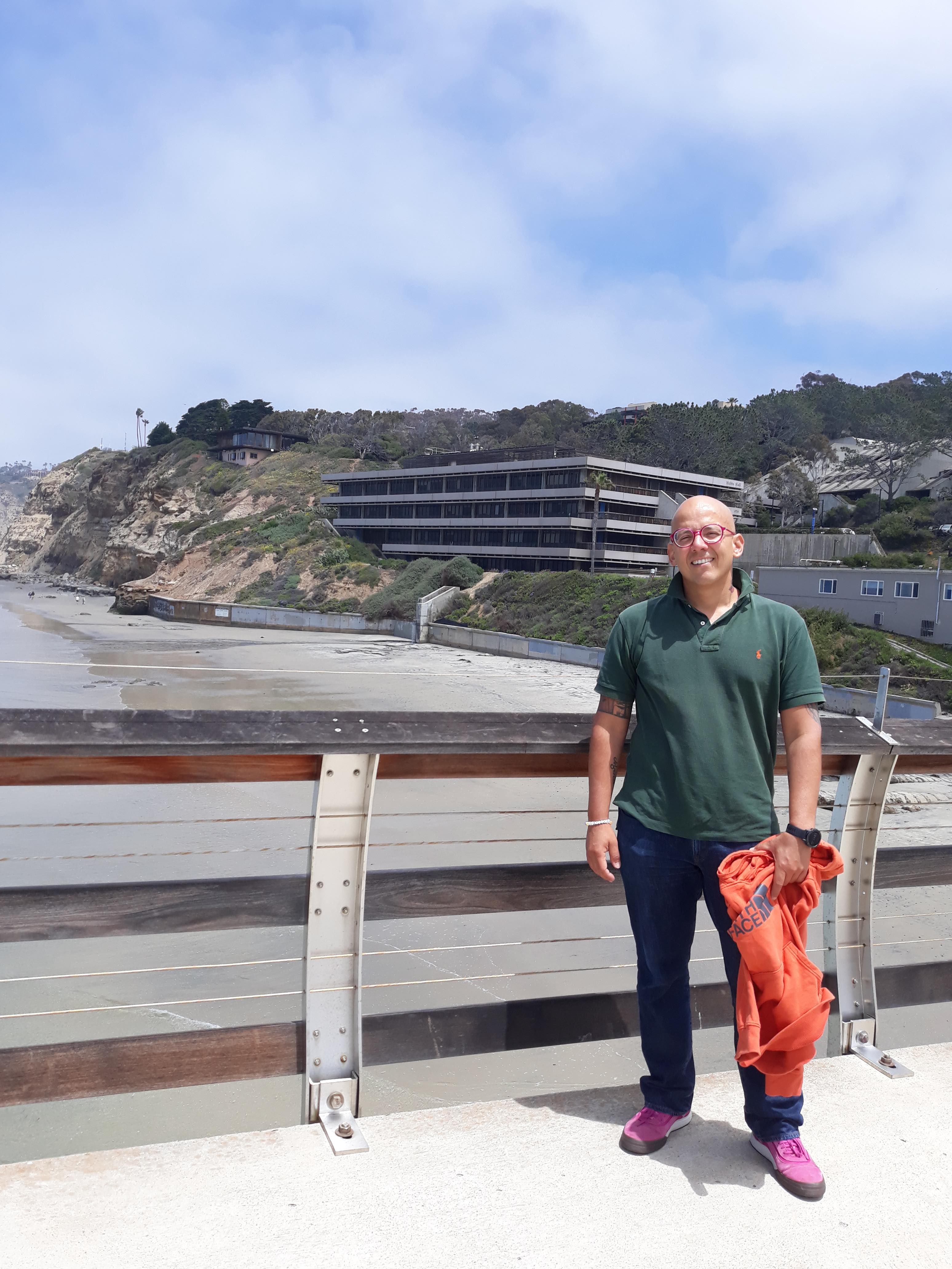
Last month I spent a few days at the Scripps Institution of Oceanography (SIO) at the University of California San Diego, as a visiting scientist to explore new avenues for research collaborations with my colleague Prof Jack Gilbert and other resident faculty at the institute.
It was a great visit packed with very fruitful scientific discussions, participation in research seminars, workshops and other activities, as well as meeting many interesting people. Not only was I able to develop potential new ideas for collaborations but I also attended interesting seminars such as a couple by Stefano Allesina, a theoretical ecologists whose work I have followed for the past decade, on the complexity and stability of complex ecosystems.
Moving from the theoretical realm I found out about the research being carried out in Dr Sara Jackrel’s lab, where she is investigating the temporal dynamics of assembly of microbial communities in the pycosphere (the microscale region surrounding phytoplankton). Interesting discussions also arose with Prof Karsten Zengler on how we could incorporate sophisticated models of metabolic networks into theoretical community ecology for a better understanding of the microbiome.
During my stay at Scripps I was also invited to participate in a new initiative for the conservation of microbes. The meeting brought together experts on many different microbial environments and ecosystems as well as conservation experts from the International Union for the Conservation of Nature (IUCN). This was an amazing opportunity to establish connections with very interesting and knowledgeable people on both these fields.
Beyond microbial conservation, Jack and I also had the chance to discuss interesting avenues for collaboration looking at the use of theoretical models to understand the temporal assembly of the gut microbiome. As part of a new project they will be conducting at SIO, an unprecedented dataset on human microbiomes followed at a very fine resolution for relatively long temporal scales will enable this understanding. We are very much looking forward to seeing how this research progresses.
Interesting synergies also arose with Dr Andrew Barton, Dr Vitul Agarwal and Dr Ewa Merz. They are studying the long-term temporal dynamics of free-living microbial communities in the ocean along the coast of California. They use a unique dataset to answer interesting questions about the temporal changes observed in marine microbial assemblages, their causes and consequences. We spent some time drawing equations on the board and thinking about how to tackle these questions from the theoretical ecology perspective.
As part of the rich set of activities I took part during my stay there I was also able to attend the PhD viva of Dr Sho Kodera. Sho is now a postdoctoral research at Gilbert’s lab and we had been in touch a few years back to discuss how theoretical models of community ecology could be put to practice to answer questions about the microbiome. This new opportunity for interaction re-sparked those old discussions and we ended up having a nice chat about potential ways in which we can mix theory and experiments of microbial assembly in the future.
With Dr Tammy Russell, we explored ideas on how to use tracking of marine birds to better understand their foraging behaviour and how this will be affected by future anthropogenic change. Our shared interest in marine birds alongside the computational tools we are currently developing at the Computational Ecology Lab to tackle issues like this created interesting synergies that we are keen to explore in the future.
All in all, a great research visit, full of interesting stories, research and friends!
None of this would have been possible without the support of the Taith International Exchange Programme and the Leverhulme Trust.
A huge thanks to Jack and his lab for the hospitality.
Conserving microbes!
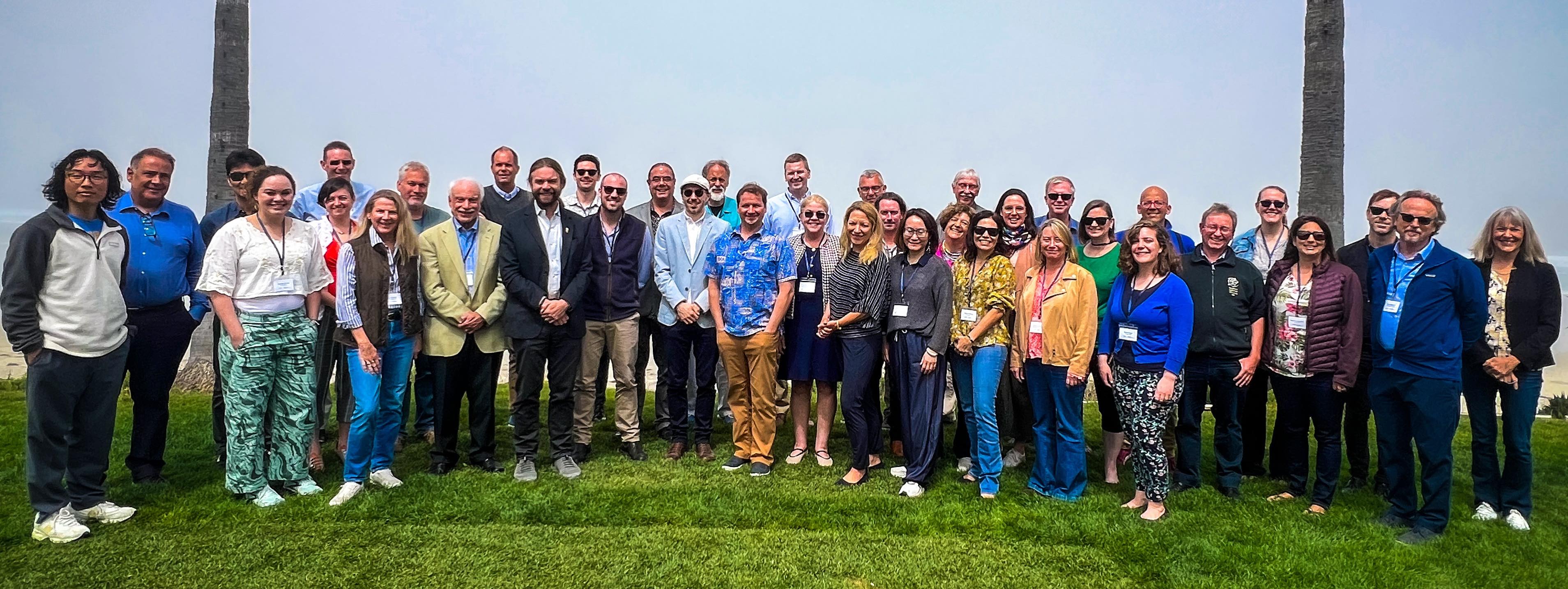
This week I was honoured with the pleasure to take part on an amazing pioneering gathering of global experts to launch a worldwide microbial conservation initiative. The meeting, held at the Scripps Institution of Oceanography in the University of California San Diego, gathered researchers from all over the world working on the most diverse threatened microbial environments as well as conservation practitioners, including representatives from the International Union for the Conservation of Nature (IUCN) and their Species Survival Commission.
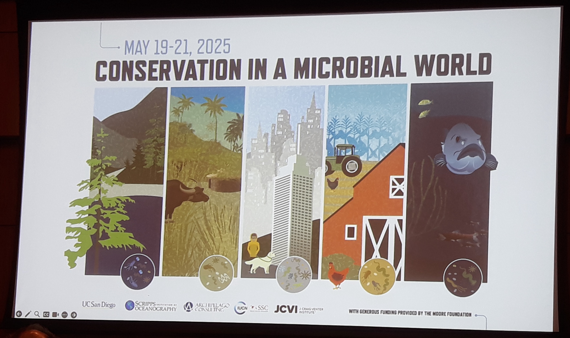
The group aims at raising awareness of the importance of conserving microbes and microbial communities, as well as developing sound strategies to achieve these goals.
As part of the meeting I had the opportunity to learn more about a diverse array of interesting microbial environments, such as the microbial mats of Cuatro Ciénagas in Mexico, an incredibly diverse microbial environment that is under threat due to different human pressures. Other interesting environments from corals, to plants and their rhizosphere, to the cryosphere (frozen environments in the Arctic and Antarctic) also took the stage, highlighting the diversity of habitats and communities that are in urgent need of conservation.
A Science correspondent joined the meeting and wrote an interesting piece about the group’s aims and objectives.
Many synergies emerged from discussions during the meeting including potential avenues to apply the theoretical ecological models we develop at the Computational Ecology Lab to the successful conservation of complex communities: microbial and macrobial!
A huge shout out to Jack and Kent for letting me part of this amazing initiative. Thanks guys!
Tropical Marine Ecology Field Course in Abu Dabbab, Egypt
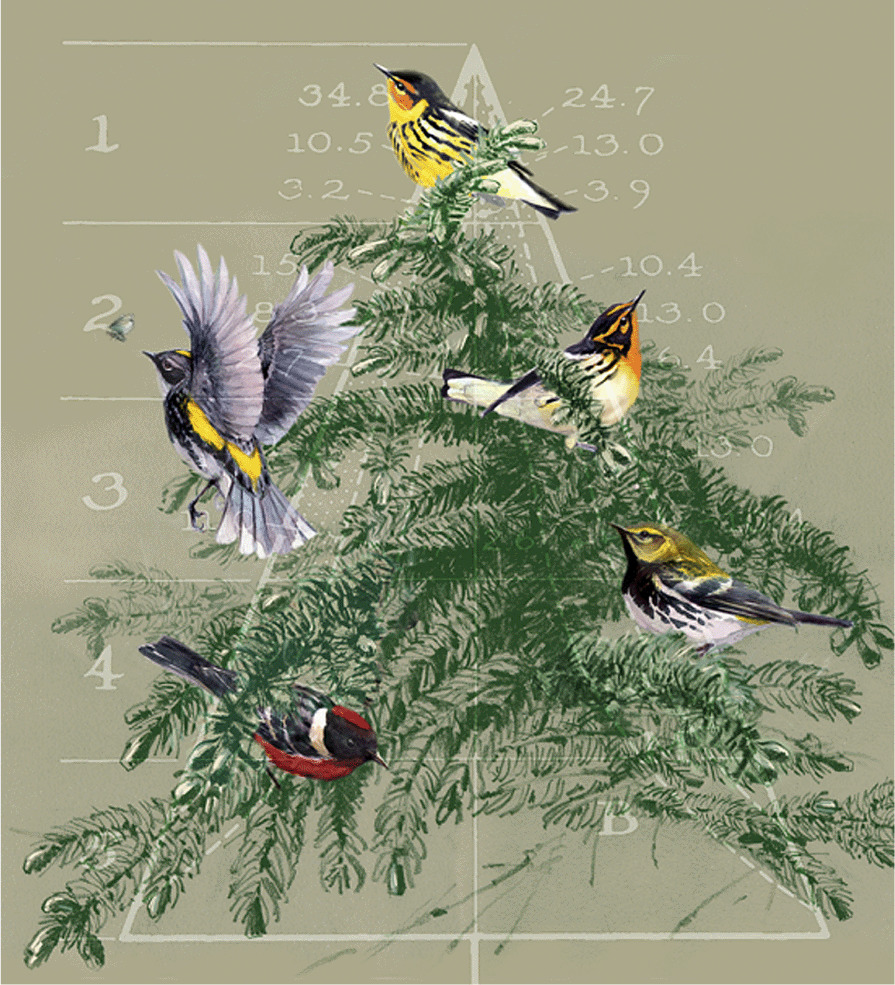
Resource partitioning is a fundamental ecological mechanism driving biodiversity. It encapsulates the idea that different species, usually closely related or belonging to the same guild, tend to exploit different resources to minimise interspecific competition and thus enhance coexistence.
The concept was originally studied in detail by Robert MacArthur in 1958 is his seminal work on warblers of the genus Dendroica (now Setophaga) in coniferous forests of the Northeastern USA. In his study, MacArthur described how 5 congeneric species from the genus Setophaga, of similar sizes and shapes and all mainly insectivorous, could coexist in the same habitat. As in turns out, the Cape May (S. tigrina), Myrtle (S. coronata), Black-throated green (S. virens), Blackburnian (S. fusca) and Bay-breasted (S. castanea) warblers are able to live together because they forage in different parts of the conifers in the temperate forests where they reside, thus potentially accessing different prey species.
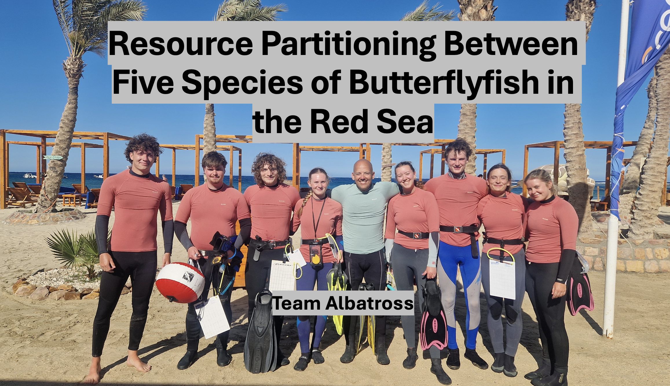
Last week, during the Tropical Marine Ecology field course in the Red Sea, I had the pleasure to help a group of keen marine biology students revisit this hypothesis in a marine system. Team Albatross, formed by Will, Alex, Neo, Leanne, Jenny, Rafe, Hannah and Rosie (from left to right in the picture) set out to study resource partitioning across 5 species of butterflyfish of the genus Chaetodon.
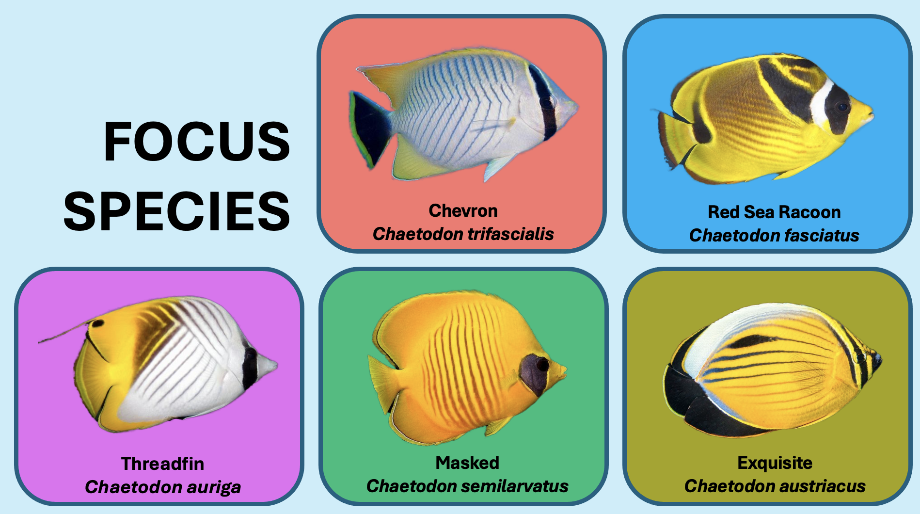
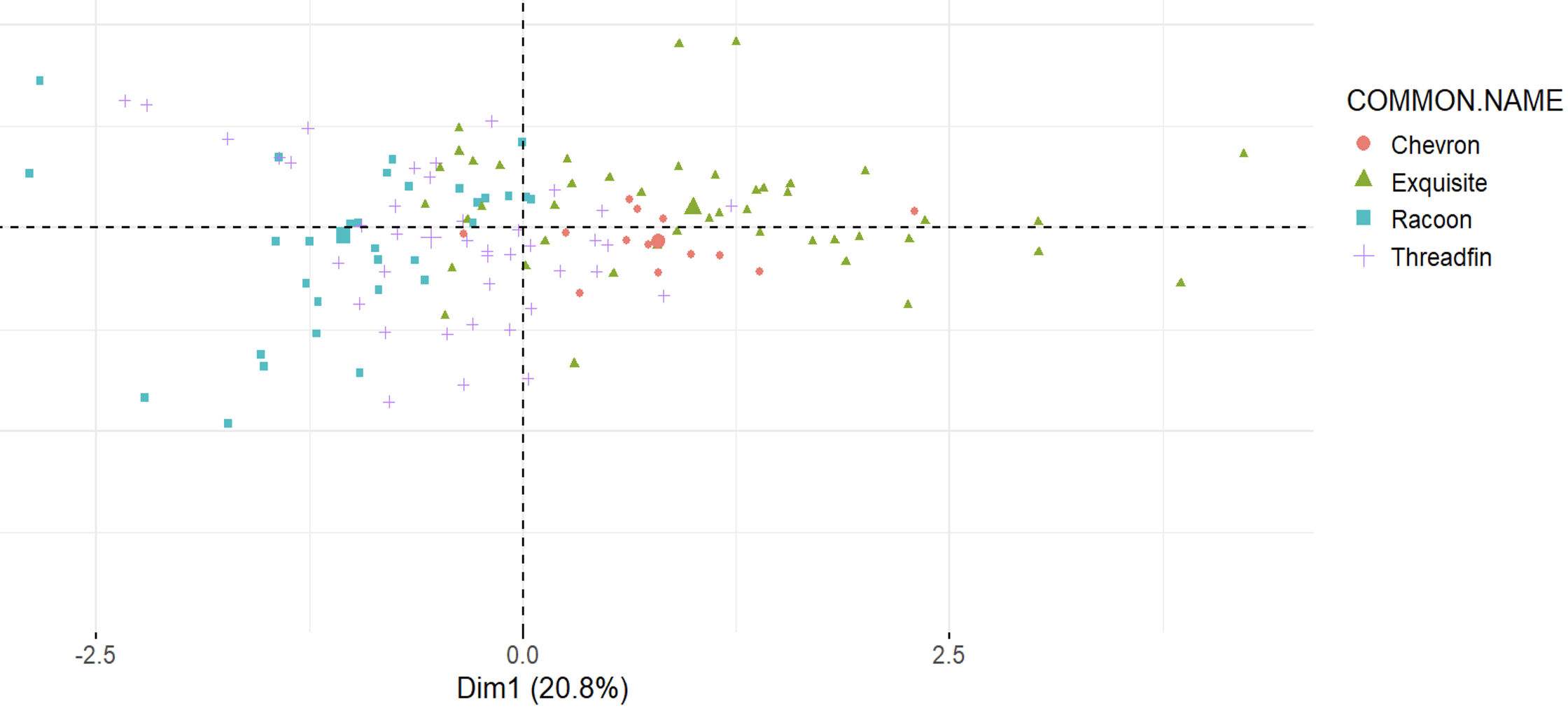
After days of intense field work, observing the behaviour of many fish across the reef of Abu Dabbab, the team was able to show resource partitioning in this genus of fish. The Threadfin (C. auriga), Chevron (C. trifascialis), Red Sea Racoon (C. fasciatus), Masked (C. semilarvatus) and Exquisite (C. austriacus) butterflyfish split their foraging efforts not only across different prey items including several species of corals, jellyfish and algae, but they also forage at different heights in the reef and at day and night.
Overall a very interesting project, loads of fun and adventure, and why not… also a little bit of thinking!
Check out our new invited talk at the Google / Alphabet Modeling Talk Series!
The link for the video recording and summary of my talk Modelling the assembly and disassembly of complex ecological systems at the Modeling Talk Series of Google / Alphabet is now live!
In this talk I presented a summary of modelling work we have been conducting at the lab over the last few years in an effort to better understand how complex species interaction networks assemble and how they respond to different perturbations from warming and invasions to habitat loss.
There are also many other interesting talks in the series that are worth checking out!