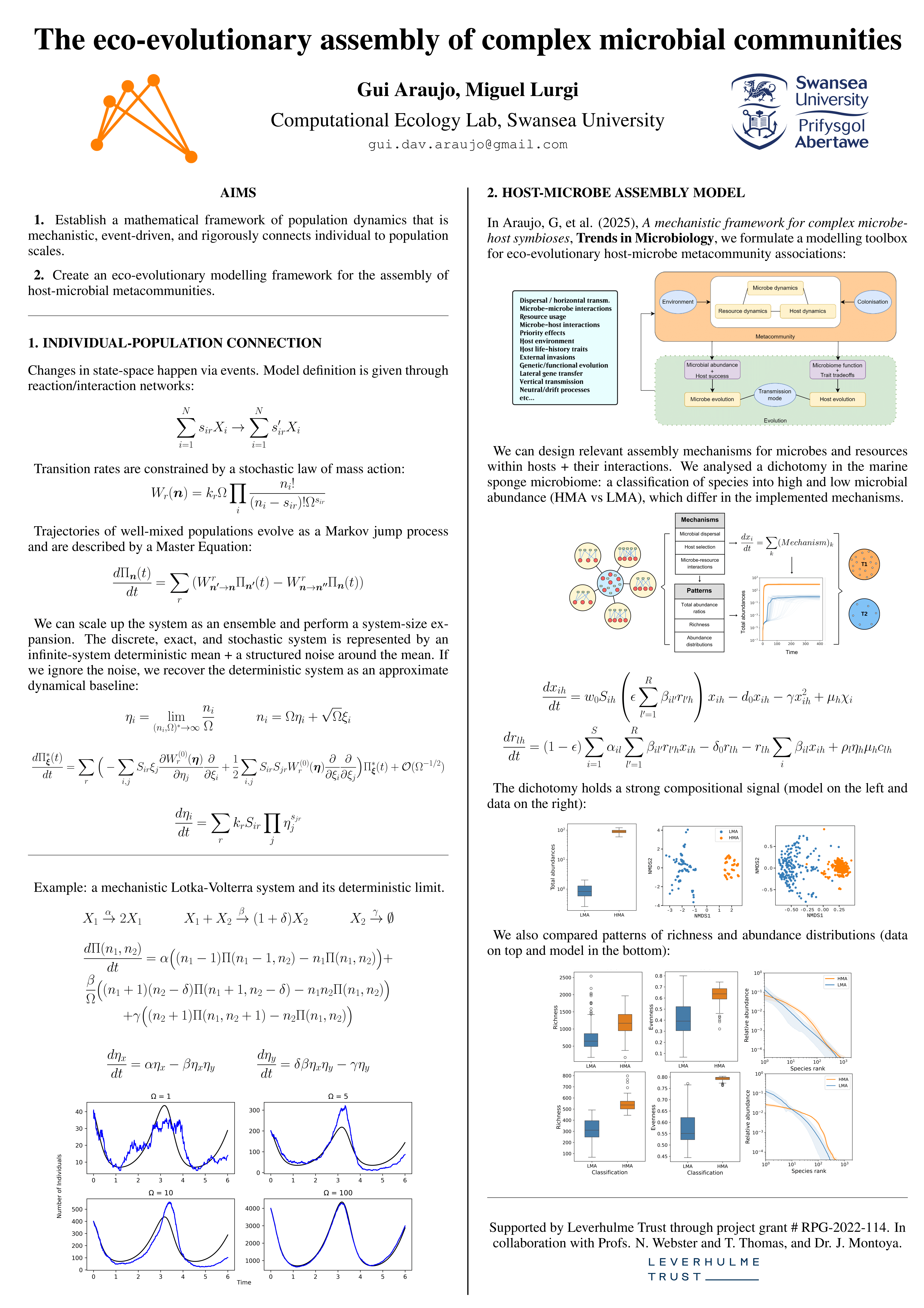
In early September, the first UK Mathematical Biology Conference took place at the University of Birmingham. Our lab was represented by Gui Araujo, who presented a poster showcasing our microbiome assembly framework.

The presentation was structured in two parts. The first focused on powerful methods from stochastic calculus that substantiate the connection between 1) specific events creating and destroying individuals and 2) global changes in densities represented by continuous flows. Many researchers at the conference work with these tools, which provided a natural entry point to discuss our extensions of the population dynamics framework. The individual-population connection is particularly relevant for the mechanistic modelling of ecological populations, since equations such as the classic Lotka-Volterra can only be directly linked to dynamics at the level of real individuals through a connection like this one. It also serves as the first step of the connections explored in our microbiome assembly framework , ultimately going through the multilayer route of individual -> population -> community -> metacommunity.
The idea behind the connection is to first establish the individual-level dynamics as a Markov jump process, described through a master equation, by modelling knowledge about events as state-dependent chances of occurrence per time step. Then, an expansion is performed on the size of the system, which increases the scope without changing the structure, going from a discrete probabilistic description to a continuous deterministic one.
The second part of the presentation featured our framework and the model we developed within it to describe microbiome assembly. This model highlights the interplay of three mechanisms: microbial dispersal, enrichment within the host environment, and microbe–resource interactions. We used this model to describe richness and abundance patterns observed in marine sponge data. Sponge species are classified into two broad categories relating to their microbiome, sponges with high and low microbial abundance (HMA and LMA). HMA and LMA sponge species differ in all three mechanisms as a consequence of their differences in pumping rates, host selection, and degree of resource allocation from host to microbes. In our (upcoming) work, we compared the model simulations with real sponge data and showed a substantial agreement between the two.
This conference was a great opportunity to engage with other mathematicians/physicists working in several fields of biology in the UK and think about how interesting it is that the same methods can be used to investigate so many different aspects of life sciences.
Participation in this conference was made possible thanks to the support of the Leverhulme Trust.

In this tutorial, Gui goes through the theoretical reasoning and calculations involved in the process of parameter estimation of a standard linear regression, starting from Bayes equation.
Here, we will derive the process of linear regression, starting from a dataset and then calculating point estimations of the parameters of a linear model using the data. Suppose we obtain a series of $N$ data points containing joint measurements of two variables, $(x_i,y_i)$, with $i=1,2,…,N$. Then, we offer a theory, a model, of how these measurements should relate to each other. In our theory, we assume that the following is true:
\[y = ax+b.\]
For this particular experiment, we don’t know the specific values of $a$ and $b$. In statistical terminology, our theory has selected a model, but has not determined it. The estimation of $a$ and $b$ that are best suited to the data we obtained is called a model determination process, as is any process of parameter estimation. The relation between $y$ and $x$ could be described by another equation, but our theory currently assumes that this is the right relation.
In order to connect data with theory, we must go through Bayes equation, which states:
\[P(Theory|Data) = \frac{P(Data|Theory)P(Theory)}{P(Data)}.\]
The logical inversion stating that
\[P(Theory|Data) \propto P(Data|Theory)\]
is a deep and powerful statement that arguably substantiates science as a whole, because it allows the conversion from knowledge about empirical observations into knowledge about our theories. However, it comes with a strong caveat: scientific theories are (of course) subjected to empirical observations, and the very usage of empirical observations is intrinsically subjected to the existence of theories. In other words, you have to give to receive. Data means nothing unless it is positioned within a theoretical frame (which, by the way, is intrinsically subjective).
So far, our theory says that $y = ax+b$ is the relation between $y$ and $x$. However, when it comes to the actual data points $y_i$ and $x_i$, they do not follow exactly this relation. The problem is: we do not get to know the true values of these variables. There are many sources of errors and limitations in our observations of these variables and, even if our model is true, we do not have access to exact measurements. Therefore, we assume that the relation in the data differs from the expected model by an error. Thus, an updated model has to be applied to the data (and not to abstract $x$ and $y$ variables), and it involves the existence of the error:
\[y_i = ax_i+b+e_i,\]
where $e_i$ is the error. In the same way as we characterised the relation between the variables (as linear) by selecting a model, we also have to characterise the error by selecting a model for its distribution. This is also a part of the assumed theory, and it can be inferred from the dataset. In the standard linear regression, on top of the linear model, we assume a normal distribution of errors (which means that this is a procedure suited for a dataset following both the facts that the variables are linearly related and the observation errors are normally distributed). Thus, we have:
\[p(e) = N(e|0,\sigma^2) = \frac{1}{\sqrt{2\pi\sigma^2}}exp\Big({-\frac{e^2}{2\sigma^2}}\Big).\]
Now, with a fully determined model, we can instantiate the Bayes equation and the statistical process:
\[P\Big(a,b,\sigma\Big|\{x_i,y_i\}\Big) = \frac{P\Big(\{x_i,y_i\}\Big|a,b,\sigma\Big)P\Big(a,b,\sigma\Big)}{P\Big(\{x_i,y_i\}\Big)}.\]
In some way, we have to compute an estimation of the parameters $[a,b,\sigma]$. However, it is necessary to bypass the dreadful factor $P\Big({x_i,y_i}\Big)$. If we follow the Bayesian route, we boldly decide to use the full posterior. The way to bypass the probability of data (or normalisation factor) is by costly sampling the posterior using tricks. The standard is an MCMC algorithm, which samples from the posterior using only kernel ratios (thus cancelling out the normalisation factor).
The classic frequentist route for the linear regression is to bypass the normalisation through an optimisation process. Instead of obtaining the full posterior, we assume uninformative (unstructured) priors and determine the mode of the posterior. This gives us the point estimation of the parameters with maximum probability given the data. In this situation, the mode of the posterior is also the mode of the likelihood, which means maximising the probability of data given the model. The likelihood is easy to calculate and easy to maximise, therefore the resulting task is to just obtain the maximum likelihood. So we start by calculating the likelihood and forgetting everything else.
The first step is to assume that the set of observed pairs ${x_i,y_i}$ is composed of independent and identically distributed points. Therefore:
\[P\Big(\{x_i,y_i\}\Big|a,b,\sigma\Big) = \prod_{i=1}^NP\Big(x_i,y_i\Big|a,b,\sigma\Big)\]
Assuming our model $y_i = ax_i+b+e_i$, we have an expression for $y_i$ given the model and also given the measurement $x_i$. Then, we can decompose each factor using the definition of conditionals:
\[P\Big(x_i,y_i\Big|a,b,\sigma\Big) = P\Big(y_i\Big|x_i,a,b,\sigma\Big)P(x_i).\]
Then, all factors $P(x_i)$ can be left out as well, since they do not depend on the model parameters (and, if we also decompose the normalisation factor in the same way, these probabilities are cancelled out). Now, the probability of $y_i$ given the other variables is given directly by the model. If the error was zero, then this probability would be $1$ if $y_i=ax_i+b$ and zero otherwise. Since we have a normally distributed error, this probability is then normally distributed around the deterministic part of the model (by definition, the error is the distribution around the deterministic value, which is then a mean):
\[P\Big(y_i\Big|x_i,a,b,\sigma\Big) = \mathcal{N}(y_i|ax_i+b,\sigma^2) = \frac{1}{\sqrt{2\pi\sigma^2}}exp\Big({-\frac{(y_i-ax_i-b)^2}{2\sigma^2}}\Big).\]
Now, substituting back into the full likelihood, we have:
\[P\Big(\{x_i,y_i\}\Big|a,b,\sigma\Big)\propto\prod_{i=1}^N \frac{1}{\sqrt{2\pi\sigma^2}}exp\Big({-\frac{(y_i-ax_i-b)^2}{2\sigma^2}}\Big)=L.\]
The structure of this function is almost begging us to work with a log transformation. Luckily, the function $log(f)$ is monotonic on $f$, so the maximum of $f$ is also a maximum of $log(f)$. Therefore, if we maximise $log(L)$, the result will be the same, and it is a much easier task. Then:
\[log(L) = \sum_{i=1}^N \Big( -log(\sqrt{2\pi \sigma^2}) -\frac{(y_i-ax_i-b)^2}{2\sigma^2} \Big)\]
\[log(L) = -Nlog(\sqrt{2\pi}) - Nlog(\sigma) - \sum_{i=1}^N \frac{(y_i-ax_i-b)^2}{2\sigma^2}\]
This is the final expression for the log-likelihood. Now, we perform the maximisation in relation to all parameters by deriving in relation to each of them and equating to zero. All expressions must be valid at the same time (consider all derivatives below as partial derivatives):
First, in relation to $a$:
\[\frac{dlog(L)}{da} = 0 = \frac{d}{da} \Big( \sum_{i=1}^N (y_i-ax_i-b)^2 \Big)\]
Then, in relation to $b$:
\[\frac{dlog(L)}{db} = 0 = \frac{d}{db} \Big( \sum_{i=1}^N (y_i-ax_i-b)^2 \Big)\]
These two equations are actually independent of omega, so they can be solved independently as a 2D system. Then, the obtained values of $a$ and $b$ can be used to determine $\sigma$ in:
\[\frac{dlog(L)}{d\sigma} = 0 = -\frac{N}{\sigma} + \frac{1}{\sigma^3}\sum_{i=1}^N (y_i-ax_i-b)^2,\]
which translates into simply
\[\sigma^2 = \frac{1}{N}\sum_{i=1}^N (y_i-ax_i-b)^2.\]
By solving the equations above for $a$, $b$, and $\sigma$, we arrive at the following expressions. First for $a$ explicitly in terms of data points:
\[a = \frac{N \sum_i (x_i y_i) - \sum_i x_i \sum_i y_i}{N \sum_i x_i^2 - (\sum_i x_i)^2}\]
Then $b$:
\[b = \frac{ \sum_i y_i \sum_i x_i^2 - \sum_i x_i \sum_i (x_i y_i) }{ N \sum_i x_i^2 - (\sum_i x_i)^2 }\]
These expressions can be prettier if we summarise them in terms of the averages of the $y_i$’s and $x_i$’s. Then, we can use $a$ and $b$ to calculate $\sigma$ from its previous equation. However, there’s an additional detail. Since we are estimating 2 parameters in this case, that expression becomes a biased estimator of $\sigma$. For an unbiased estimation, we must discount the 2 degrees of freedom from the variance, and the expression then becomes:
\[\sigma = \sqrt{ \frac{1}{N - 2} \sum_{i=1}^N (y_i - ax_i-b)^2 }\]
If we run a standard linear regression as a statistical test, for example the function lm() in R, we are not only calculating the point estimates of the parameters as above. The parameter $\sigma$ is reported as a residual standard error (RSE), and R also includes estimations of the errors on the parameters that are calculated from the estimated $\sigma$, the parameter standard errors. We are also performing t-tests for the null hypotheses of $a$ or $b$ being equal to zero, and that is where p-values enter. Diagnostic statistics of residuals (such as their distribution summaries) are also provided to assess model assumptions like normality and homoscedasticity.

Last month I spent a few days at the Scripps Institution of Oceanography (SIO) at the University of California San Diego, as a visiting scientist to explore new avenues for research collaborations with my colleague Prof Jack Gilbert and other resident faculty at the institute.
It was a great visit packed with very fruitful scientific discussions, participation in research seminars, workshops and other activities, as well as meeting many interesting people. Not only was I able to develop potential new ideas for collaborations but I also attended interesting seminars such as a couple by Stefano Allesina, a theoretical ecologists whose work I have followed for the past decade, on the complexity and stability of complex ecosystems.
Moving from the theoretical realm I found out about the research being carried out in Dr Sara Jackrel’s lab, where she is investigating the temporal dynamics of assembly of microbial communities in the pycosphere (the microscale region surrounding phytoplankton). Interesting discussions also arose with Prof Karsten Zengler on how we could incorporate sophisticated models of metabolic networks into theoretical community ecology for a better understanding of the microbiome.
During my stay at Scripps I was also invited to participate in a new initiative for the conservation of microbes. The meeting brought together experts on many different microbial environments and ecosystems as well as conservation experts from the International Union for the Conservation of Nature (IUCN). This was an amazing opportunity to establish connections with very interesting and knowledgeable people on both these fields.

Beyond microbial conservation, Jack and I also had the chance to discuss interesting avenues for collaboration looking at the use of theoretical models to understand the temporal assembly of the gut microbiome. As part of a new project they will be conducting at SIO, an unprecedented dataset on human microbiomes followed at a very fine resolution for relatively long temporal scales will enable this understanding. We are very much looking forward to seeing how this research progresses.
Interesting synergies also arose with Dr Andrew Barton, Dr Vitul Agarwal and Dr Ewa Merz. They are studying the long-term temporal dynamics of free-living microbial communities in the ocean along the coast of California. They use a unique dataset to answer interesting questions about the temporal changes observed in marine microbial assemblages, their causes and consequences. We spent some time drawing equations on the board and thinking about how to tackle these questions from the theoretical ecology perspective.
As part of the rich set of activities I took part during my stay there I was also able to attend the PhD viva of Dr Sho Kodera. Sho is now a postdoctoral research at Gilbert’s lab and we had been in touch a few years back to discuss how theoretical models of community ecology could be put to practice to answer questions about the microbiome. This new opportunity for interaction re-sparked those old discussions and we ended up having a nice chat about potential ways in which we can mix theory and experiments of microbial assembly in the future.


With Dr Tammy Russell, we explored ideas on how to use tracking of marine birds to better understand their foraging behaviour and how this will be affected by future anthropogenic change. Our shared interest in marine birds alongside the computational tools we are currently developing at the Computational Ecology Lab to tackle issues like this created interesting synergies that we are keen to explore in the future.
All in all, a great research visit, full of interesting stories, research and friends!
None of this would have been possible without the support of the Taith International Exchange Programme and the Leverhulme Trust.
A huge thanks to Jack and his lab for the hospitality.
