Miguel Lurgi
06 March 2026
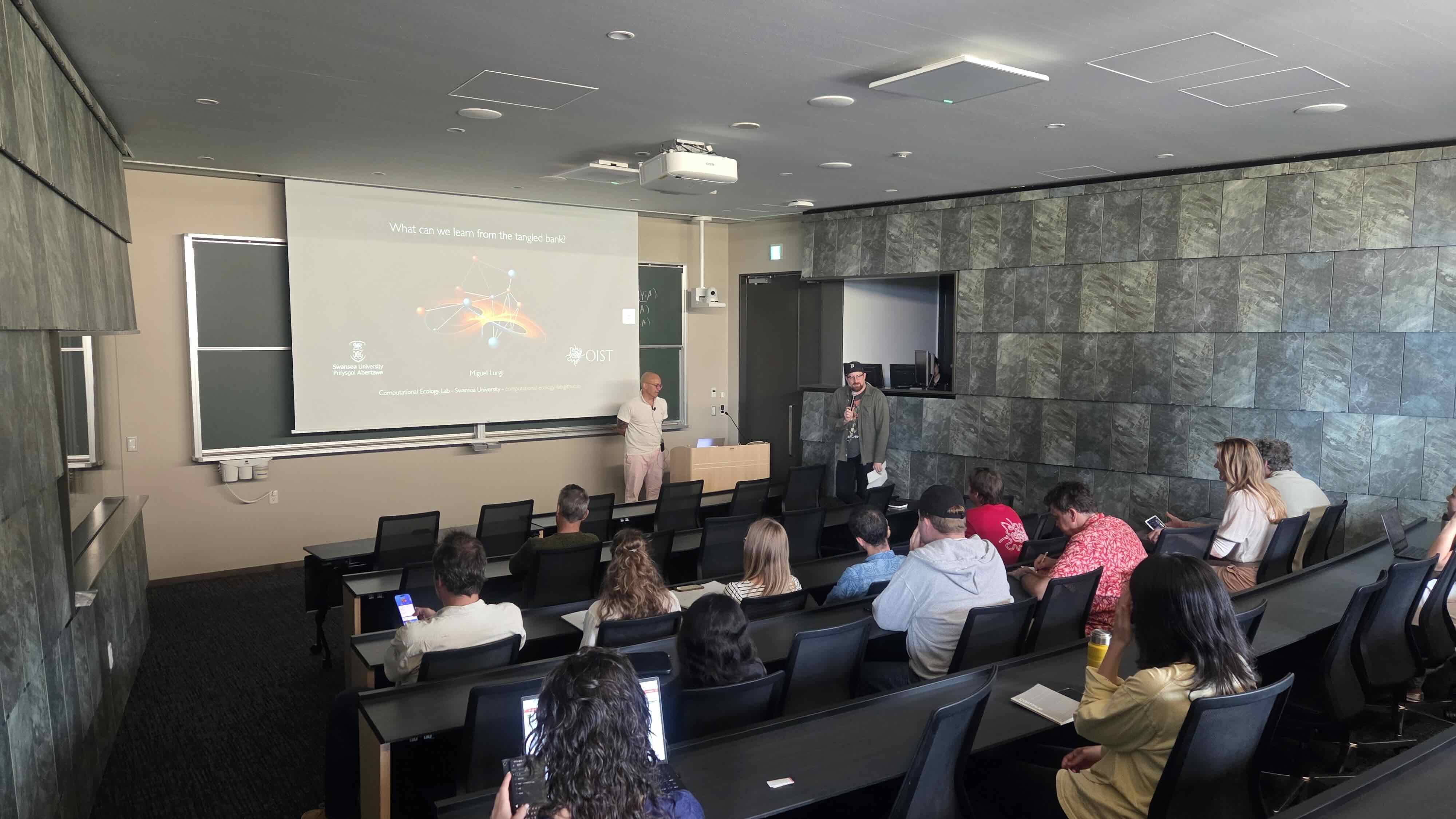
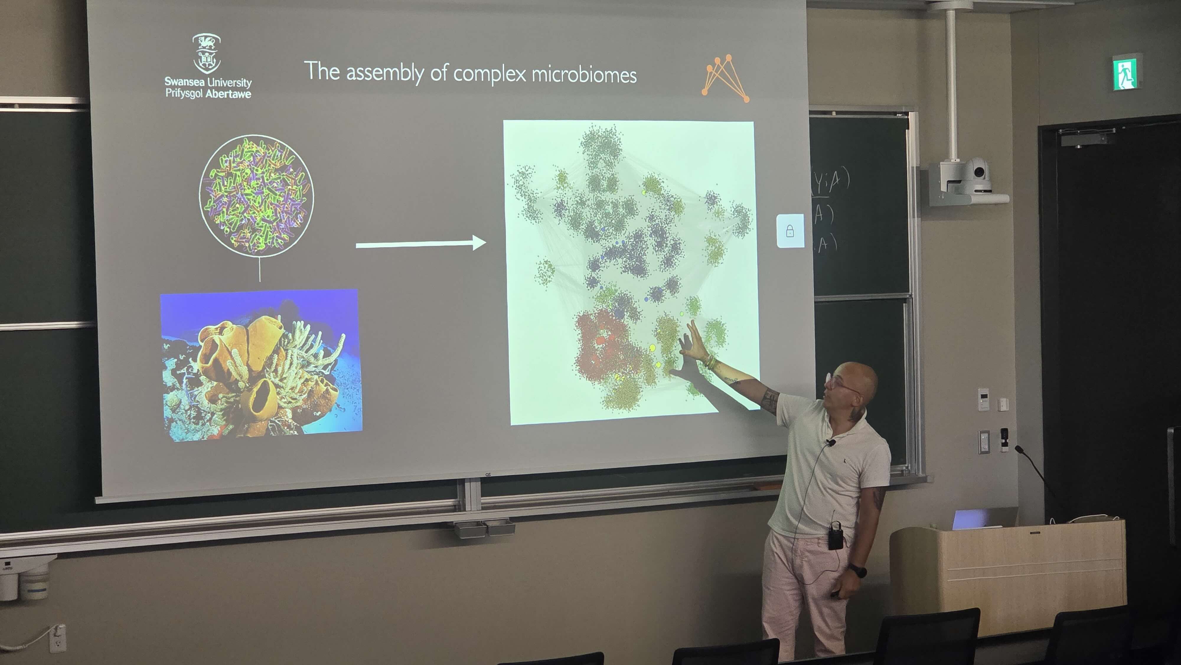
Today I did my invited general audience seminar at the Okinawa Institute of Science and Technology (OIST) entitled: What can we learn from the tangled bank? The network organisation of ecological systems. After a very nice introduction by Dave Armitage, head of the Integrative Community Ecology Unit at OIST, I went right into business and gave an overview of the work we have done, and continue to do, in the lab. I drew on examples from our work on spatial scaling, terrestrial avian food webs, and the microbiome all within the context of classical ecology from Hutchinson and the niche to May and ecosystem stability. Towards the end of the talk I also presented our recent work on the eco-evolutionary dynamics of complex networks with multiple interaction types.
At the end of the talk there were many thought-provoking questions and further discussions sparked by the talk. As a result I will continue discussing this during my time left at OIST with students and staff members who expressed interest in our work!
Special thanks of course go to my friend and collaborator Nuria (Galiana), and my PhD students and postdoc: Abby, Lucie, and Gui, without whom none of what I presented would have been possible. And of course thanks to the TSVP for organising!
The research I presented in this talk was partly funded by the Leverhulme Trust.
Miguel Lurgi
27 February 2026
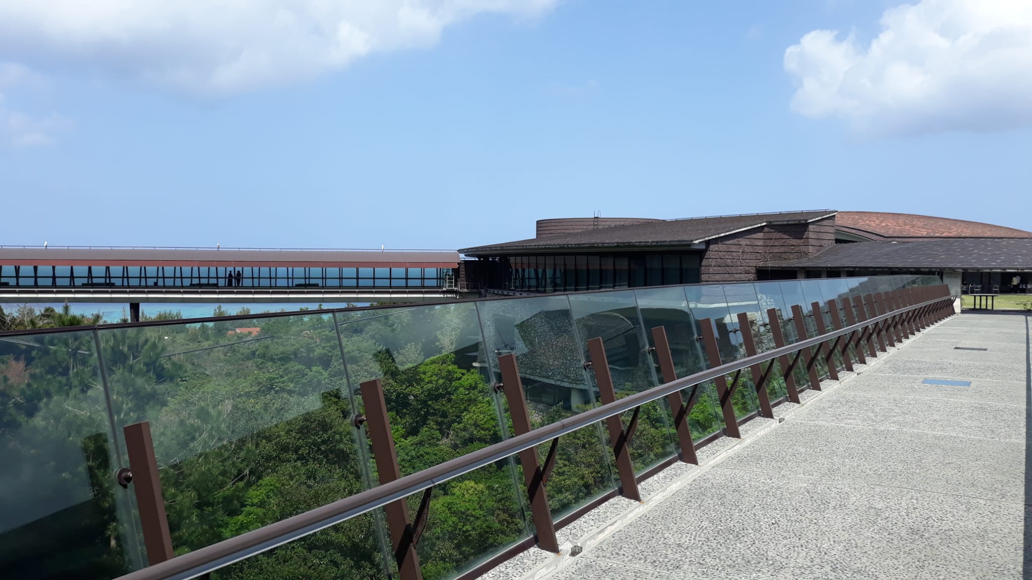
This year, for a few months, I am developing my research at the Okinawa Institute of Science and Technology (OIST), a truly amazing place to conduct interdisciplinary research and experience the Japanese culture.
So far, I have had the opportunity to interact with many scientists working on very interesting topics from the physics of phase transitions in Cacio e Pepe pasta to the philosophical implications of current and short term future developments of artificial superintelligence.
Resident researchers have been very welcoming. I have been given the chance to showcase my research at the Ravasi and Armitage units lab meetings. I have also had very interesting discussions on the behaviour of complex dynamical systems, the effects of disturbances on the response diversity of complex ecosystems, how to look a the dynamics of ranks to better understand community compositional changes, all the way to the functional and genetic richness of the marine environment. All this in the inspiring atmosphere of cutting edge research facilities and a great scientific environment.
I have also joined a team of scientists in the field, visiting some interesting research sites part of the Okinawa Environmental Observation Network (OKEON) that monitors, among other things, the soundscape of Okinawa’s habitats. Using their acoustic monitoring, scientists at OIST can understand changes in community composition. Excitingly, we have been thinking together how to build networks of interactions between bird species and how their structure is affected by environmental conditions. I’m excited to see where that research direction takes us.
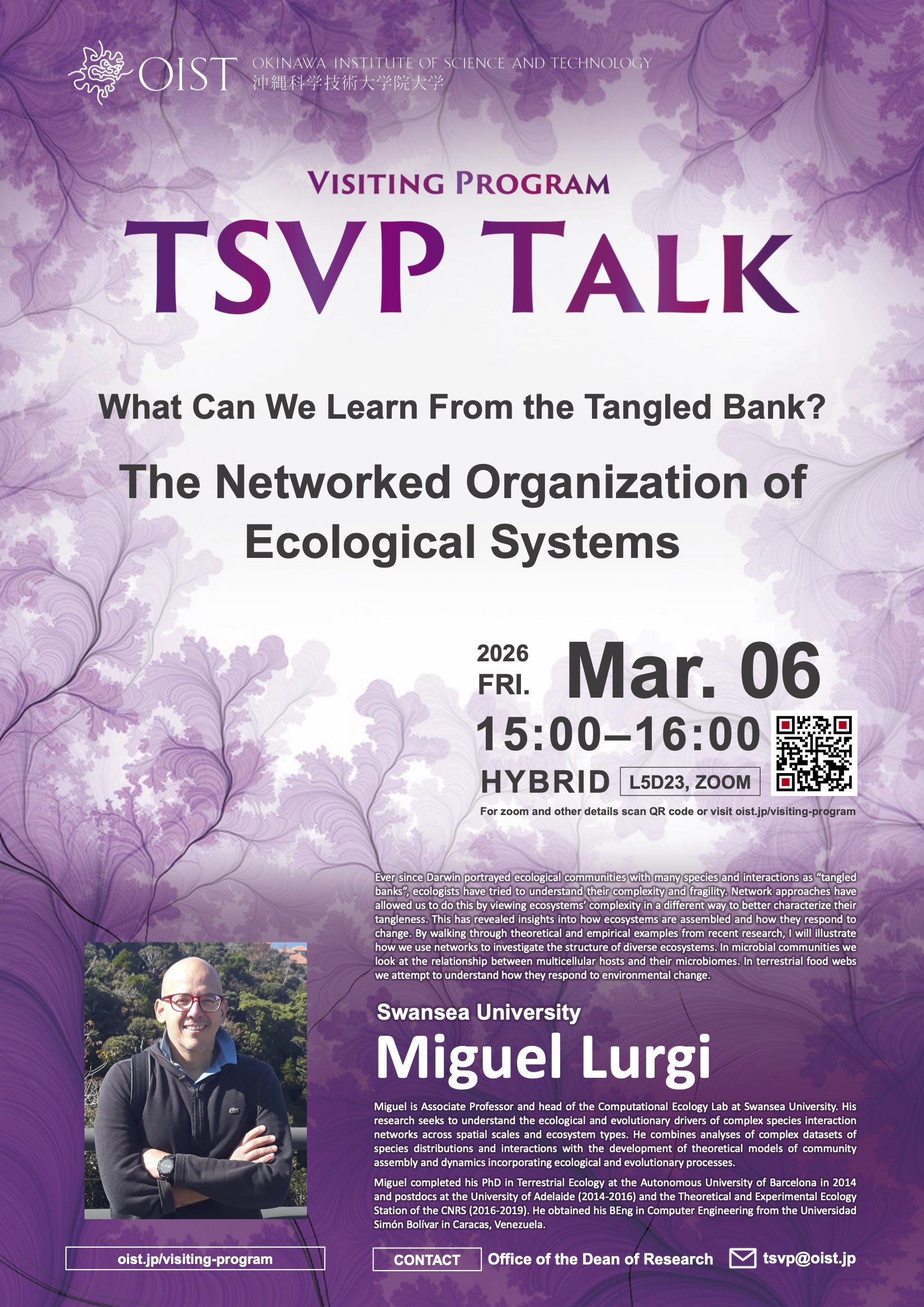
As part of the programme that made my visit possible, the Theoretical Sciences Visiting Program I have been invited to give a talk about the research with do in the lab for general audiences. So, on Friday 6th of March I will talk about: What can we learn from the tangled bank? The networked organisation of ecological systems.
I’m very much looking forward to sharing our research with the staff and students at OIST!
And of course, it is always nice to take some time to enjoy other activities. People are super friendly in Okinawa, and they have welcomed me warmly in their basketball and baseball teams as well as taking me around to do some diving and birdwatching around the island - including seeing a few lifers :)
I’m very grateful to everyone at OIST for making my time so enjoyable so far. I’m looking forward to the rest of my visit!
Miguel Lurgi
16 December 2025
This week I once again had the pleasure to share the lab’s research with scientists from around the world at the Annual Meeting of the BES, this year in Edinburgh!

With countless interesting talks and posters, thematic sessions and just the vibrant atmosphere, this meeting is always a chance to catch up with friends and colleagues on the latest developments of our research and have fun while doing it. This year, I also contributed in other ways by joining a focus group where we discussed the impact of the Annual Meeting on our research and on ecological science. Thanks Rachel for the chance to join this group!
I also chaired a session on Evolutionary Ecology: Plasticity, dispersal and ecological responses which was full of interesting talks and discussions from the impact of adaptive dispersal on population persistence to the evolution of sex ratios in breeding systems.
During my poster presentation on the Coevolutionary drivers of phylosymbiosis and microbiome divergence in host-microbe associations, I had the chance to discuss with several interesting people our ideas on the origins of complex symbioses and how we can develop quantitative mathematical models to better understand them.
Before heading back to Swansea I had some time to check out the Christmas market and other nice sightings in the city centre of Edinburgh. A very nice town! And of course, to head down to the pub, or catch up at the venue, with old friends from all over the world.
Thanks to the Leverhulme Trust (through project grant RPG-2022-114) for the support to attend and present my work at this meeting.
Miguel Lurgi
29 November 2025
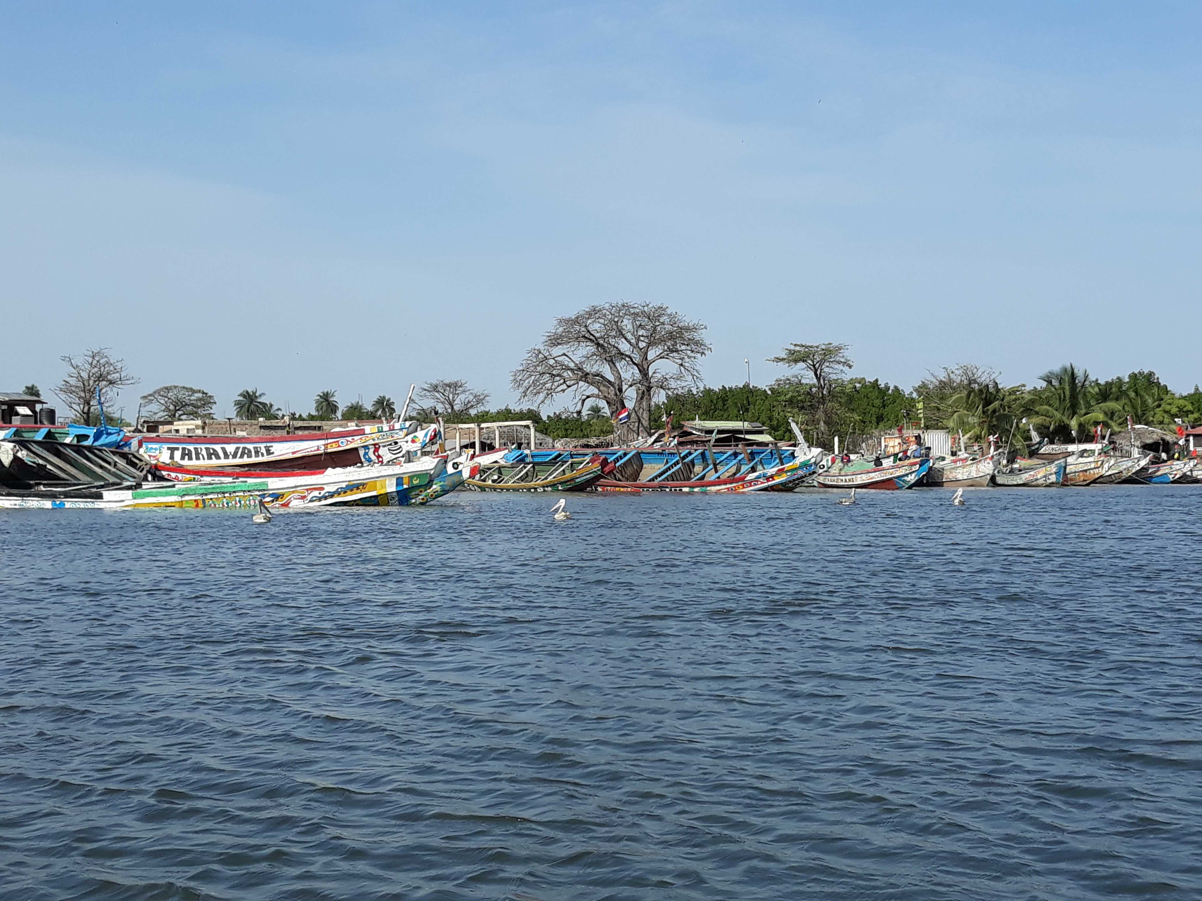
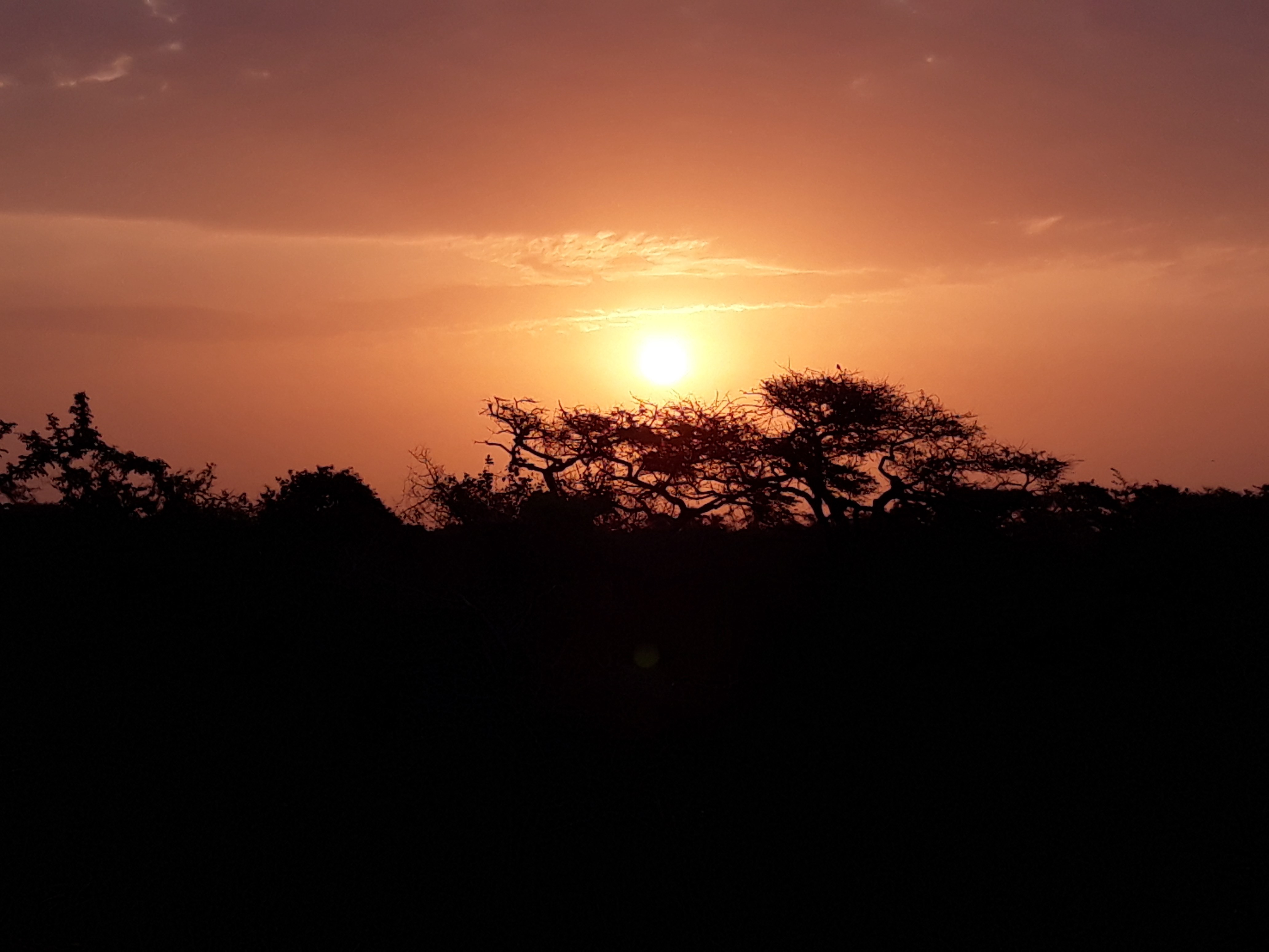
For a few days this November I was very lucky to be part of a research expedition to the Kartong Bird Observatory in The Gambia. I had the opportunity to learn more about the projects they are running from the population genetics of a couple of species of vultures (Hooded Necrosyrtes monachus and White-backed Gyps africanus) to the migration patterns and wintering ecology of nightingales Luscinia megarhynchos. Many inspirational ideas emerged from this for potential future research projects at Kartong touching the applied side of the research we develop at the Computational Ecology Lab.
The expedition was a success, with around 3450 individual birds from 154 different species recorded. These data constitute a valuable contribution to bird research in The Gambia and more generally for a better understanding of bird populations worldwide.
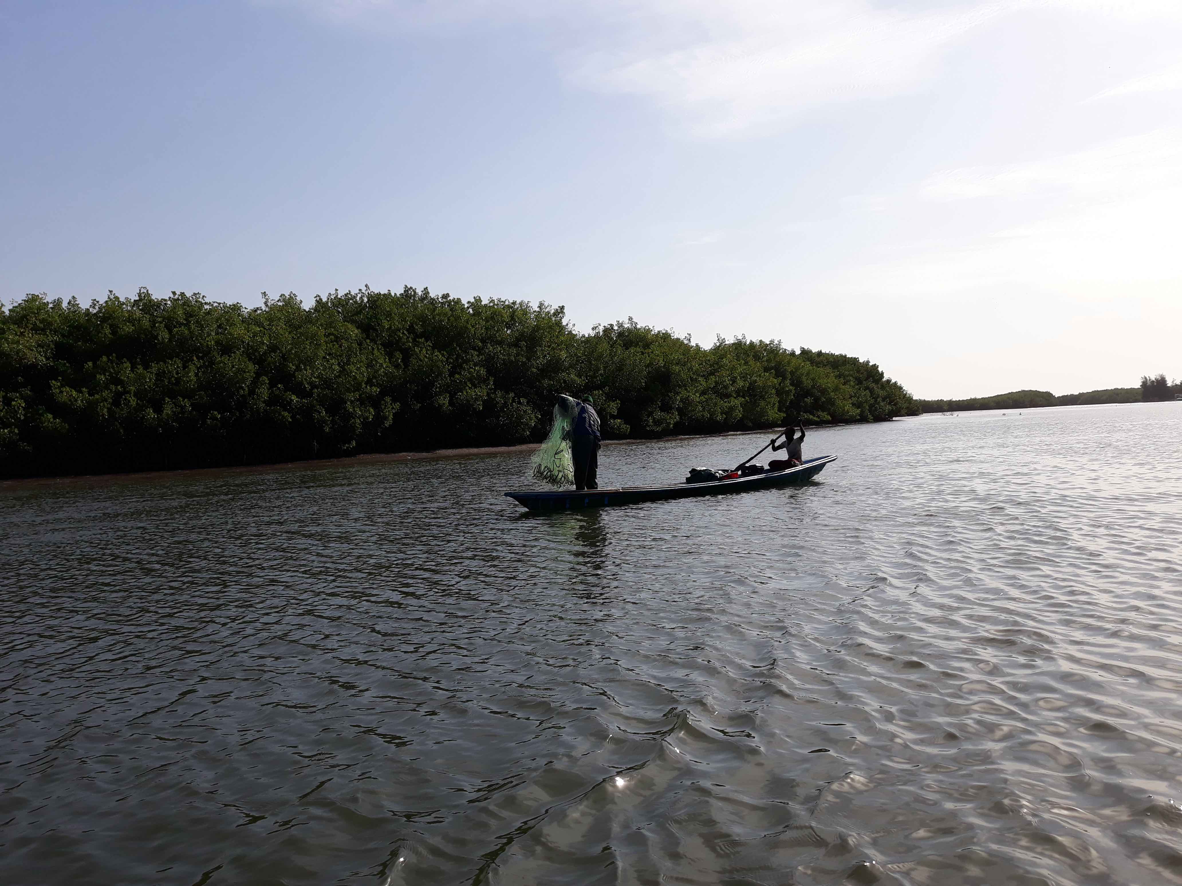
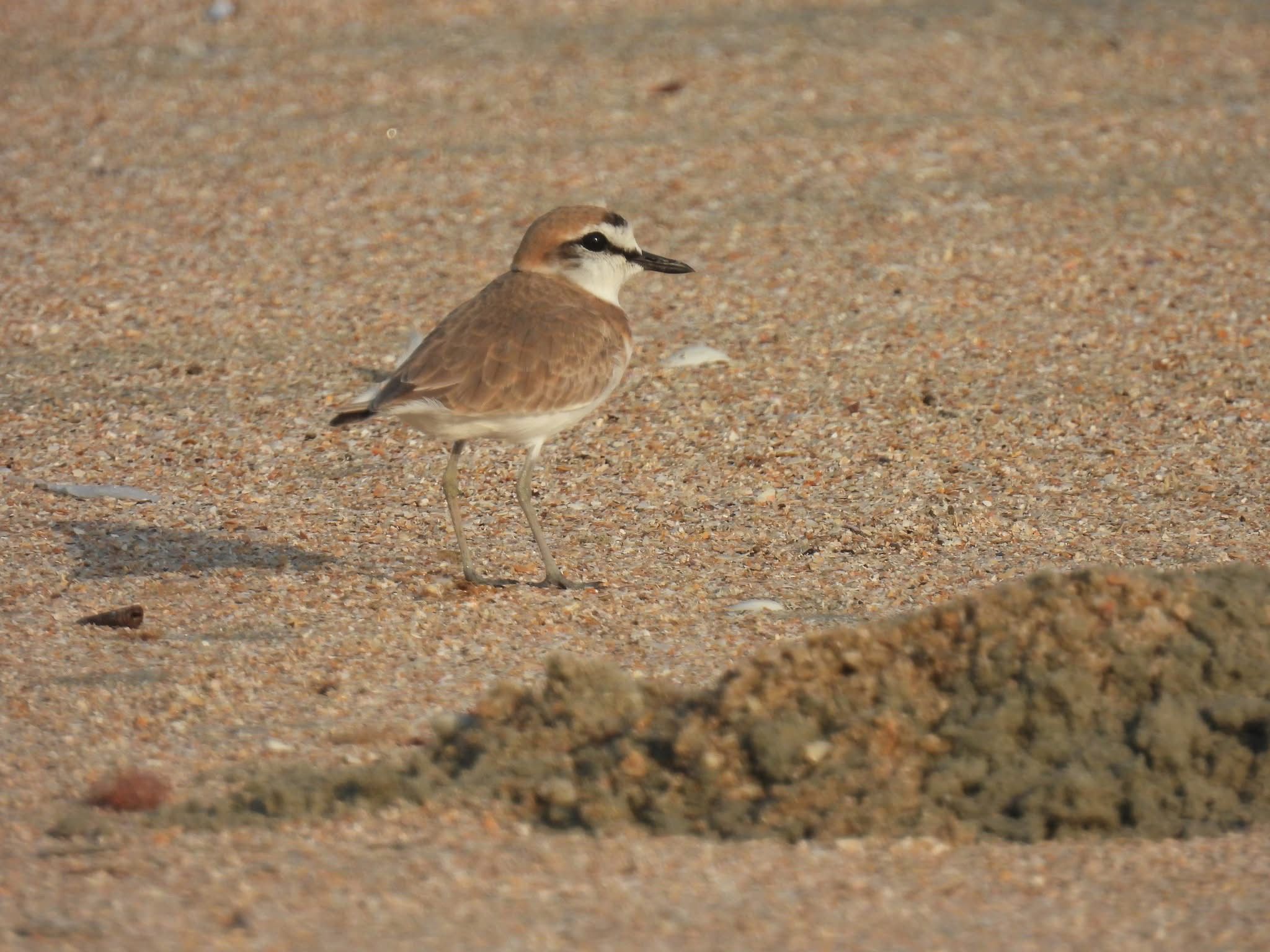
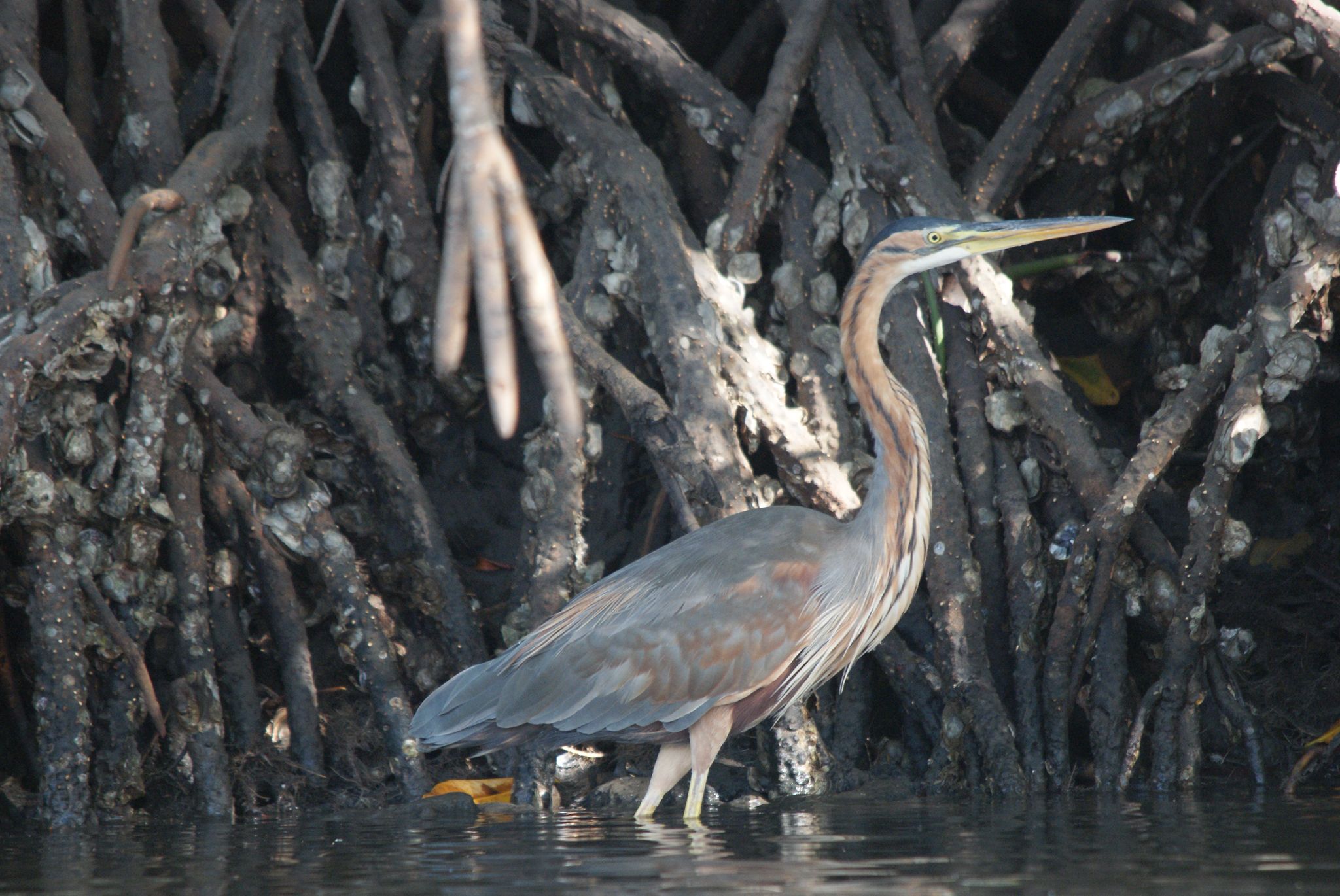
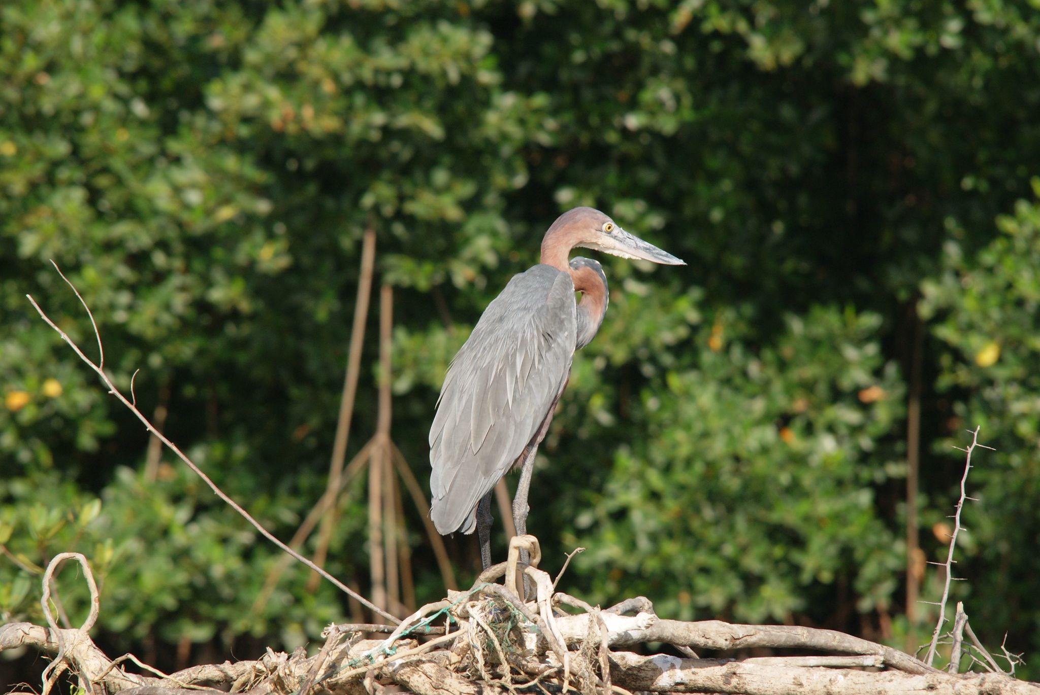
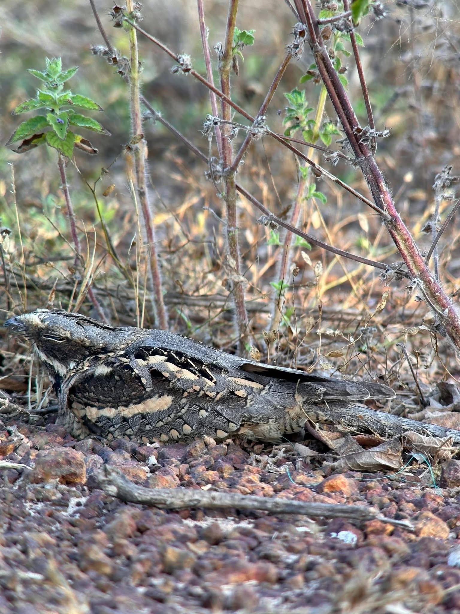
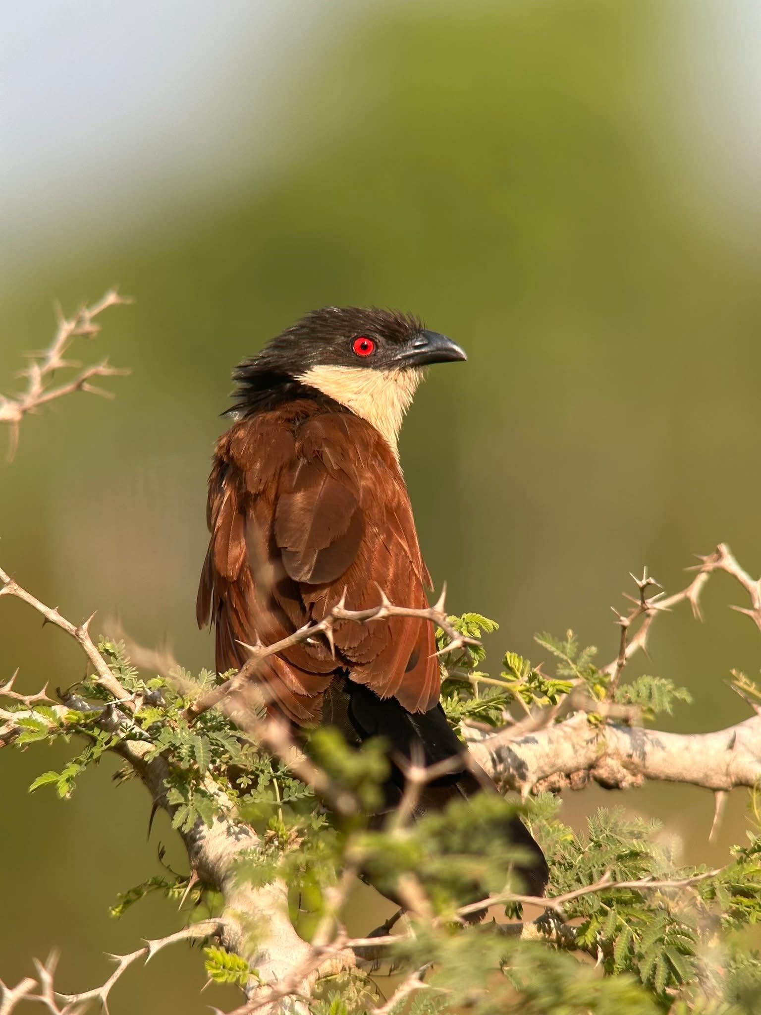
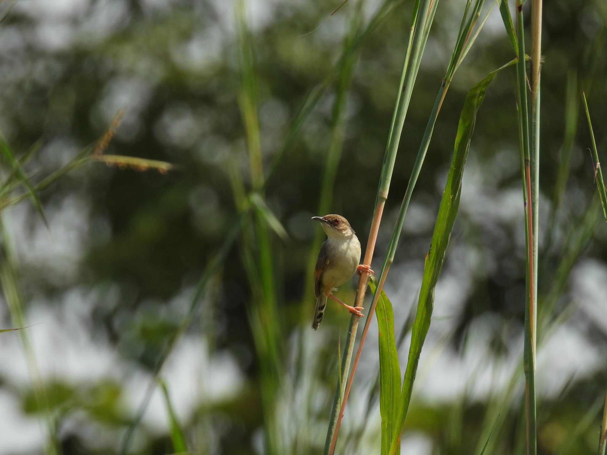
As an added bonus I enjoyed very much the ringing and the birdwatching, with so many species observed in amazing habitats. I had the opportunity to join ringing teams both on terrestrial as well as wetland and estuarine environments. Everyday presented new chances to see and experience different locations and different species, from the massive flocks of Western Reef Egretta gularis, Black Egretta ardesiaca, Striated Butorides striata, Squacco Ardeola ralloides and Black-headed Ardea melanocephala herons that roamed the grasslands of Batabar, to the Grey Pluvialis squatarola, Common Ringed Charadrius hiaticula and White-fronted Charadrius marginatus plovers as well as Whimbrels Numenius phaeopus and Common Actitis hypoleuca, Green Tringa ochropus and Wood Tringa glareola sandpipers of the coastal and mangrove habitats of Barracunto and Stala. Not to mention the beautifully coloured birds found across the entire reserve such as Little Merops pusillus, Blue-cheeked Merops persicus and Swallow-tailed Merops hirundineus bee-eaters, Yellow-crowned Gonoleks Laniarius barbarus, Senegal Coucal Centropus senegalensis, Beautiful Sunbird Cinnyris pulchellus, Red-cheeked Cordonbleu Uraeginthus bengalus amongst many others!

On the personal side, beyond the ringing, it was great to get to meet and interact with an incredible team of researchers and expert ornithologists such as Michael, Emmanuel, Naffie, Olly, Roger, and many others. I am really grateful for their guidance and the knowledge imparted during the expedition. It was great to be part of the team.
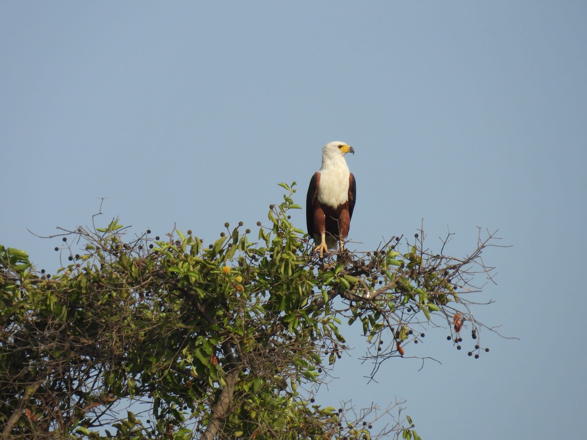
I had an amazing time as part of the Swamp Squad, paddling around puddles and getting into deep ponds for which my thigh waders were not enough! Always in the search for nice species such as White-faced whistling ducks Dendrocygna viduata, Greater Painted-snipe Rostratula benghalensis, and of course Ospreys Pandion haliaetus!
Thanks to all the team for an unforgettable experience and especially to the Swamp Squad, my bro Billy who was always making the time enjoyable, and the people of Kartong! Hope to be back soon.
Photo credits: Purple Heron, Goliath Heron and Crocodile kindly provided by Laura Raven and John. White-fronted Plover, Long-tailed Nightjar, Senegal Coucal, Singing Cisticola and African Fish Eagle kindly provided by Noelia D. Alvarez and Ricki McCloud. Thanks for letting me use your pictures guys!
Miguel Lurgi
03 November 2025
Today I had the pleasure to share my research on the modelling of complex ecosystems across scales with the researchers and students at the School of Biosciences of the University of Sheffield.

In my talk on Cross-scale community assembly: from microbiomes to spatial food webs, I presented some of our recent findings on the eco-evolutionary theoretical framework we are developing to unveil the origins of complex symbioses. I then moved on to larger ecological scales and discussed some results on the spatial modelling of complex food webs and the effects of perturbations on their stability and organisation.
Before heading back to Swansea I had some time to check out the pair of peregrine falcon around St George’s church!
I would like to thank Oscar for the kind invitation and for organising the visit. Also, to Andrew and his group for the great discussions and the great dinner out after the seminar. Hope to visit again soon!