Modelling Coffee: Noise-induced effects in collective dynamics
In this tutorial, Marco explains how to implement the main routines to replicate the effects of the paper on Noise-induced effects in collective dynamics and inferring local interactions from data
Part 1 Gillespie algorithm
The code contains a function for exactly simulating runs from the master equation through the Gillespie algorithm. The Gillespie algorithm is divided in four main parts:
1.- Find the velocity (or propensity) for every reaction. This is done by multiplying the reaction rate (which is conditioned on the reagents encountering each other) with the rate that the reagents do encounter each other. The rate that two reagents encounter each other can be found through the mass action assumption. Usually this is done simply by multiplying the concentration of the reagents, but this is an approximation that holds only for big population sizes because reagents do not interact with themselves, and the concentration of the species with and without one molecule can be quite different in small population sizes and omega. Hence it is possible to use the stochastic law of mass action, equal for one reaction to $ k \Omega \prod \frac{x_i!}{(x_i-1)! \Omega^{s_i}} $ (for details see David Schnoerr et al (2017) J. Phys. A: Math. Theor. 50, 093001). Since there are some factorials, it is hard to compute in practice, and has been rearranged in the code implementation.
2.- Find the waiting time before the next reaction occurs by sampling from an exponential distribution with mean rate equal to the sum of the reaction velocities.
3.- Find the reaction that happens by choosing from the possible reactions with a probability proportional to the reaction velocity.
4.- Update the states based on the reaction that happened.
The function has not been optimized but works for simulating every type of system starting from the microscopic reactions. It performs only one update and must be inserted inside a for loop for producing the entire simulation. As input, it requires:
1.- The current number of molecules/individuals in a specific state through a vector of size equal to the number of possible states and each entry the number of individuals in that state.
2.- A vector containing the reaction rates.
3.- A matrix indicating the stoichiometry of the reagents, with the number of rows equal to the number of reactions, and number of columns equal to the number of possible states, and entries equal to the number of species of that state that must encounter to produce the specific reaction.
4.- A matrix indicating the stoichiometry of the products, with the number of rows equal to the number of reactions, and number of columns equal to the number of possible states, and entries equal to the number of species of that state that are produced from that specific reaction.
5.- A parameter omega indicating the spatial scale of the system.
As output, it gives a vector containing the waiting time, the number of the reaction the occurred, and the new number of individuals/molecules in each state.
It could be a good test to modify the code to simulate clonal logistic growth by using these reactions: A -> 0 with rate 0.05, A -> 2A with rate 0.2, 2A -> A with rate 0.05. You can start multiple replicates by having only one individual and set omega to 50.
Part 2 Replication of the results of the paper “Noise-induced effects in collective dynamics and inferring local interactions from data”
The replication of the results consists of two parts, one applied to the voter model, and one applied to the higher order interactions model (see the paper for details). The only difference between the two is that the higher order interactions also has a reaction of the type 2A + B -> 3A, which leads to a non-linear per capita rate of change in the ordinary differential equation and consensus formation with multi-stability in the limit of infinite population size (not present in the voter model). For each model it is shown examples of the dynamics through 20 replicates of the time series obtained iterating the Gillespie algorithm and the probability density of the population being in certain states. Interestingly, also the voter model shows consensus and multi-stability! This is because of the constructive effect of intrinsic noise. To better understand this result, it is possible to fit a Langevin equation to the time series we have simulated and find the functional form of the deterministic (drift) and stochastic (diffusion) terms. Despite the Langevin equation being an approximation, it explicitly defines a term for stochasticity, enabling us to investigate noise, quite cool.
To fit the data, we first have to find the autocorrelation function for figuring out the best time scale (see paper for details).
\[ACF(\tau) = \frac{\langle (M(t) - \langle M(t) \rangle ) (M(t+\tau)- \langle M(t) \rangle) \rangle}{\langle (M(t) - \langle M(t) \rangle)^{2} \rangle }\]When I see an equation my first though is “how do I calculate that?”. In my opinion Tidyverse has some cool operations which can be used to translate the equation into a specific value. For example, the averages in the ACF are calculated over different things, which can be captured by grouping.
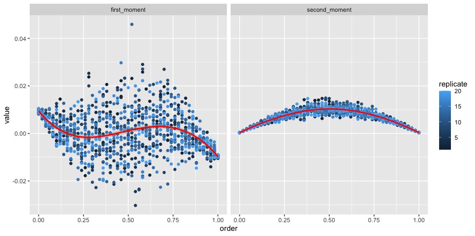
The last part is to find the deterministic and stochastic component, which produce respectively the first and second moments (see paper for details). The first moment is the average “jump” from a specific population state. The second moment is the variance of such “jumps”. In this case there are only two possible individual states, only one degree of freedom to describe the state of the entire population, but in more complex cases a “jump” could be a vector in a multidimensional state space.
Comparing the two models we see that the deterministic component “pushes” the population towards non-consensus in the voter model (equal number of individuals for both options), while there are two stable equilibria separated by and unstable equilibrium in the higher interaction model (equilibria are found when the “push” is equal to zero, and equilibria are stable when the “push” goes towards the equilibrium). For both models the noise is stronger when the population is undecided because there is more uncertainty in the reactions that can occur (the reactions have similar velocities), which is the definition of intrinsic noise. Hence, the voter model is pushed away from its non-consensus equilibrium condition, leading to noise induced consensus. Noise constructs order!
Marco has kindly share his code with us here.